Brownian Motion

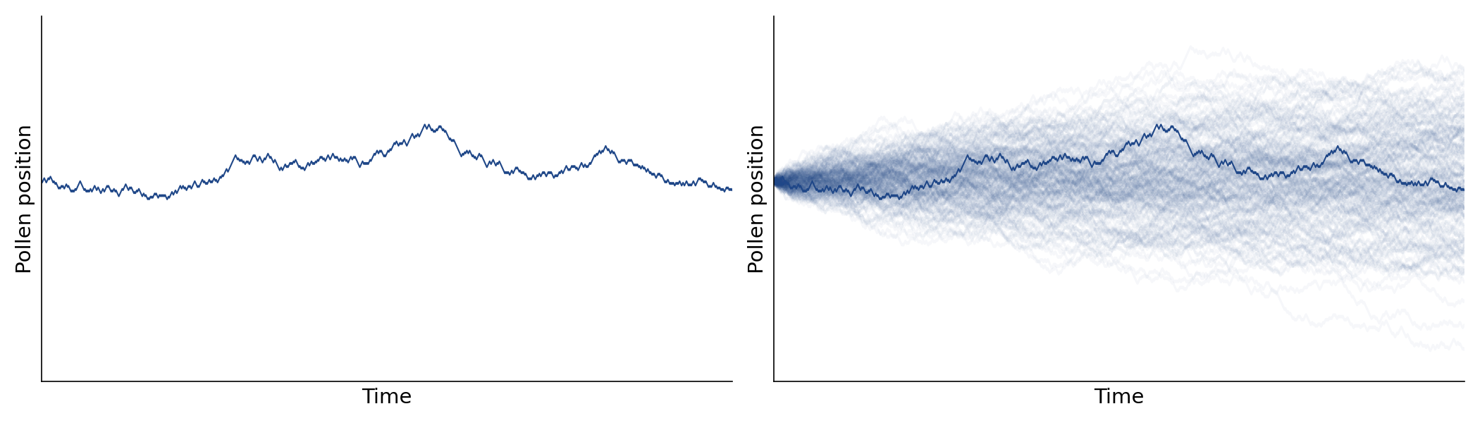
Imagine that a pollen particle is suspended in a glass of water. If we were to observe and record the vertical position of the particle over time, we would find that its movements were random. And if we were to plot this position, we’d get a jagged path through time (Figure $1$, left). This path would be just one of many possible paths, and if we were to repeat this observational experiment many times, we would not expect to see the same path again.

Given this randomness, how can we reason about this phenomenon? Can we say anything interesting or useful about the particle? For most of human history, this was a seemingly impossible task. A key insight, a conceptual pillar in probability theory, is to separate what actually happened (Figure $1$, left) from other possible outcomes (Figure $1$, right). This approach allows us to reason about the world through counterfactuals: what are all the possible paths the pollen could have taken? How likely is each path? What can we say about the distribution of outcomes?

Figure 1. Left. A single random path of a pollen particle's vertical position plotted against time. Right. Many such random paths, all starting at the same initial position.

This understanding of the pollen particle as a random process is a deep idea, and it took many decades and scientists to understand. The phenomenon was first observed in the 1830s by the Scottish botanist Robert Brown. Brown used a microscope to observe pollen particles suspended in water, and to his surprise, he saw the particles moving! At first, he thought this meant that the pollen particles were alive, but he tested and then rejected this hypothesis by observing the same effect with particles that he was convinced were inanimate, such as glass powder, minerals, and even pulverized fragments of the Egyptian Sphinx (Góra, 2006)! For roughly half-a-century, the phenomenon remained a mystery, although it became known as Brownian motion.

Then starting in 1905, Albert Einstein published a series of papers in which he hythesized that the pollen particles were moving because they were being bombarded by invisible molecules in the liquid (Einstein, 1905). In the following year, the Polish physicist Marian Smoluchowski independently published essentially the same theory (Von Smoluchowski, 1906). At the time, this theory was controversial, because the idea of molecules was not yet widely accepted. However, using statistical mechanics, Einstein and Smoluchowski were able to make testable predictions about the behavior of the particles, and another scientist, Jean Baptiste Perrin, verified the model a few years later (Perrin, 1909). And since Einstein’s breakthrough work, Brownian motion has been widely studied and more deeply understood. In the mathematical community, Brownian motion was formalized by Norbert Wiener (Wiener, 1923), and thus Brownian motion is often referred to as a Wiener process, particularly by mathematicians.

The goal of this post is to better understand Brownian motion. Brownian motion is an important concept because it can be used to model many phenomenon, from particles suspended in liquids to the prices of stocks. Ultimately, we’ll reconstruct the marginal distribution of our pollen particle at any given point in time. As we will see this, this is the normal distribution. This deep connection means that we can make mathematically precise probabilistic statements about a completely random process.

Random walks

Let’s begin with a simplified model of our pollen particle in discrete time. This is a stochastic process called a random walk. In the next section, we’ll extend this to continuous time, which is Brownian motion.

Imagine we can discretize time and then observe a single discrete “tick” on the clock. What happens to the pollen particle during this one tick? In our simple model of the world, we’re going to imagine that we flip a coin, not necessarily fair, and that the pollen particle moves up or down the same amount based on the outcome of that coin toss. The coin toss models the fact that the pollen particle is being randomly bombarded by water molecules and thus its position at the next time point is random. So the pollen particle cannot stay in place; after one tick of the clock, it moves up or down.

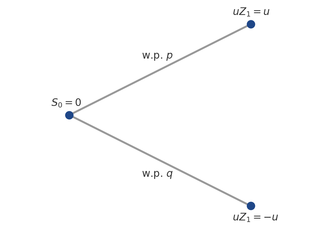
Formally, let $S_0$ be the particle’s initial position (non-random), and let $S_1$ be a univariate random variable denoting the vertical position of the pollen particle after one tick. We assume that the initial position is zero ($S_0 = 0$), since this makes our calculations and notation easier and since it is simply a vertical shift in the final path. So we flip a coin with bias $p$, where $p$ is the probability of heads ($H$) and $q := 1-p$ is the probability of tails ($T$). If the coin is heads, then the pollen particle moves up $u$, and if the coin is tails, then the pollen particle moves down $u$ (to $-u$). Let’s denote the outcome of each coin flip as a random variable $Z_i$, taking values in $\{-1, 1\}$. Then the position after a single coin flip is $u Z_1$ (Figure $2$).

Figure 2. A one-period model of a pollen particle. After a coin clip which is heads with probability $p$, the pollen particle moves either up to $u$ or down to $-u$. $S_0$ denotes the initial position, and $u Z_1$ denotes the position after the coin flip.

Now consider the position $S_n$ after $n$ time steps. At each time point $i$, we flip a coin, which we assume is independent of all other coin tosses, to discover whether the pollen particle is displaced up or down from its current position. Then $S_n$ is simply the sum

$S_n = u Z_1 + u Z_2 + \dots + u Z_n. \tag{1}$

Since each $Z_i$ is random, $S_n$ is also random.

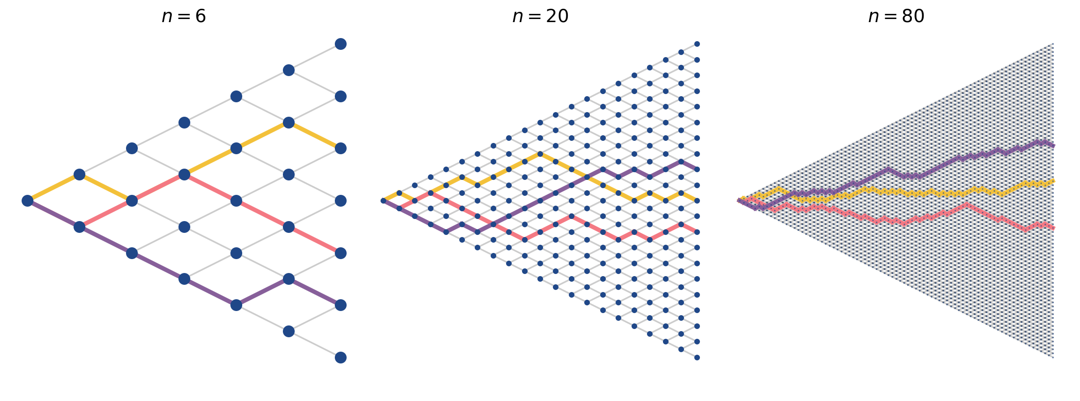
Clearly, as we repeatedly flip our coin, the set of possible locations of the pollen particle expands linearly with $n$. We can visualize all these possible locations as a directed graph or tree, sometimes called a binomial tree (Figure $3$, left)—we’ll explain the name in a moment. The tree layers (vertical slices) are zero-indexed, and so the root node occurs at time $n=0$. Each node is a possible location, and the $n$-th layer is all possible locations by time $n$. The directed edges (left to right) are valid moves of the pollen particle. A path in this binomial tree is a sequence of steps which starts at the tree’s root (left-most node) and continues right at each time step until it reaches a leaf node (right-most node). A valid path is one that always moves left-to-right, from root to leaf. A valid path cannot, for example, move straight down at the same time point or move backwards.

Figure 3. Left.A binomial tree with depth $n=5$. Each node is labeled with the net number of up or down moves required to reach that node. Two random paths are shown in yellow and red. Right. The left plot but with the nodes labeled with $(n,k)$ tuples, indexing the number of coin filps and thus the possible number of endpoints by that many flips.

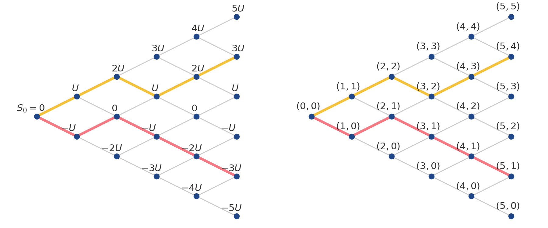
To help us identify nodes, let’s introduce the counting number $k$, which indexes the leaf nodes, taking values in $k \in \{0, 1, \dots, n\}$. Like the time index $n$, the number $k$ is a zero-based index. Let’s denote the bottom leaf node with $k=0$ and the top leaf node with $k=n$. To illustrate this, I’ve visualized the tree with the nodes labeled with tuples $(n, k)$ (Figure $3$, right).

Now that we understand this simple, discrete-time model for our pollen particle, let’s tackle our motivating question: which outcomes (leaf nodes) are most likely? Any given path is random, but can we say something about the distribution of outcomes?

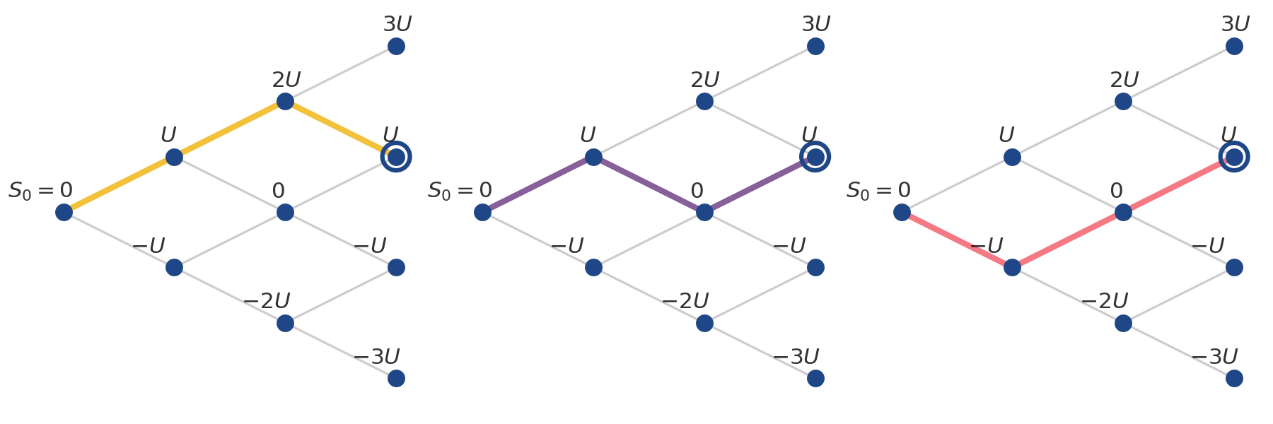
To start, let’s compute the probability of arriving at the highlighted leaf node in Figure $4$. This is really the probability of arriving at a given node $(n, k)$, which in turn is really the probability of flipping $k$ heads in $n$ coin tosses. Let’s use $K_n$ for this random variable. Arriving at this node requires that we flip two heads and one tails. The probability of this is

$\mathbb{P}\left(\{ \text{two heads and one tails} \}\right) = p^2 q. \tag{2}$

However, there are three ways flip two heads in three coin tosses,

$\{ HHT, HTH, THH \}, \tag{3}$

which is another way of saying that there are three paths to the highlighted node. Since each path is a mutually exclusive outcome, we compute our desired probability by summing the probability of all outcomes in Equation $2$ by the number of paths:

$\mathbb{P}\left(\{ \text{arriving at node $(3, 2)$} \}\right) = \mathbb{P}(K_3 = 2) = 3 p^2 q. \tag{4}$

For example, if $p=1/2$, then this probability would be $3/8$.

Figure 4. A binomial tree of depth $n=3$. There are three possible paths (red, yellow, purple) to arrive at the node $(3, 2)$ (circled node).

To compute this probability in general, we just need a way to compute the number of ways to get $k$ successes or heads in $n$ trials. Since order matters, the number of ways to pick $k$ heads from $n$ coin tosses is

$n (n-1) (n-2) \dots (n-k+1) = \frac{n!}{(n-k)!}. \tag{5}$

First, we can choose any of $n$ coin tosses to be a heads. Then we can pick any of $n-1$ coins tosses to be heads. And so on, until we have $k-1$ heads. (The last pick is completely constrained.)

However, this overcounts the possible paths. For example, this does not distinguish between $H_1 H_2$ and $H_2 H_1$, where the subscript $i$ denotes the $i$-th coin toss. So we need to divide the permutation in Equation $5$ by the number of ways we can order elements in a $k$-sized set. This is $k$ factorial. Putting this together, we see that the number of ways to get to each node in the binomial tree is

$\frac{\text{ordered ways to pick $k$ heads from $n$ tosses}}{\text{permutations of $k$ heads}} \;\; = \;\; \frac{n(n-1)(n-2) \dots (n-k+1)}{k(k-1)(k-2) \dots 1}. \tag{6}$

This number in Equation $6$ is often called the binomial coefficient, pronounced “$n$ choose $k$”, and is denoted as

${n \choose k} \triangleq \frac{n!}{k! (n-k)!} \tag{7}$

Putting it all together, the probability of arriving at the $k$-th node in the $n$-th layer of a binomial tree is

$\mathbb{P}(\{K_n = k\}) = {n \choose k} p^k q^{n-k}. \tag{8}$

The fact that these probabilities sum to one is just a trivial application of the binomial theorem. See A1.

Computing the mean and variance of $K_n$ is relatively straightforward. We can view $K_n$ as the sum of independent Bernoulli random variables, so

$K_n = \frac{Z_1 + 1}{2} + \frac{Z_2 + 1}{2} + \dots + \frac{Z_n + 1}{2}. \tag{9}$

The mean of each $Z_i$ is $2p - 1$, and the first two moments are easy to compute:

$\begin{aligned} \mathbb{E}[K_n] &= \sum_{i=1}^n \mathbb{E}\!\left[\frac{Z_i + 1}{2}\right] = np, \\ \mathbb{V}[K_n] &= \sum_{i=1}^{n} \mathbb{V}\!\left[\frac{Z_i + 1}{2}\right] = npq. \end{aligned} \tag{10}$

For the variance calculation, we use Bienaymé’s identity and the fact that $(Z_i+1)/2$ are independent. The distribution of $K_n$ was first discovered by Jakob Bernoulli and is called the binomial distribution after the binomial terms implicit in $n$ choose $k$—again, see A1—and hence the “binomial tree.”

Of course, $K_n$ is the distribution on the number of heads in $n$ coin tosses, while we’re more interested in the location of the pollen particle. But there’s a simple relationship between the two. The location $S_n$ is simply the number of up moves ($K_n$), minus the number of down moves ($n - K_n$), scaled by the size of the move $u$. In other words, it is:

$\begin{aligned} S_n &= u \left( Z_1 + Z_2 + \dots + Z_n \right) \\ &= u \left(K_n - (n - K_n)\right) \\ &= u \left(2 K_n - n\right). \end{aligned} \tag{11}$

Since $n$ and $u$ are non-random, the events $\{S_n = u(2k-n)\}$ and $\{K_n=k\}$ are identical. So we can say

$\mathbb{P}(\{S_n = u(2k-n)\}) = \mathbb{P}(\{K_n = k\}) = {n \choose k} p^k q^{n-k}. \tag{12}$

So the location of our pollen particle by a given layer $n$ is determined by the distribution of a random variable $K_n$ with the probability mass function (PMF) in Equation $8$. While $K_n$ and $S_n$ have the same probabilities, they clearly have different moments. The first two moments of $S_n$ are:

$\begin{aligned} \mathbb{E}[S_n] &= \mathbb{E}[u(2K_n - n)] = 2nu(p-1/2), \\ \mathbb{V}[S_n] &= \mathbb{V}[u(2K_n - n)] = \mathbb{V}[2 u K_n] = 4 u^2 npq. \end{aligned} \tag{13}$

In the special case in which $p = 1/2$, then

$\begin{aligned} \mathbb{E}[S_n] &= 0, \\ \mathbb{V}[S_n] &= n u^2. \end{aligned} \tag{14}$

We can explore this distribution by plotting the function for various parameterizations (Figure $5$). Note that while $K_n$ is binomially distributed and while $S_n$ and $K_n$ have the same probability function, $S_n$ is not binomially distributed. That’s because the binomial distribution only has support over the non-negative integers. It’s a distribution over repeated coin flips. But $S_n$ has support over the negative numbers. I don’t think the distribution of $S_n$ has a name, but speaking loosely, it is essentially a binomial distribution mean-centered at zero.

Figure 5. The distribution of the position $S_n = u(2K_n - n)$, where $K_n \sim \text{binom}(n, p)$. In the context of the binomial tree, these represent the distribution of locations $S_n$ of our pollen particle at time slices $n=6$, $n=20$, and $n=80$.

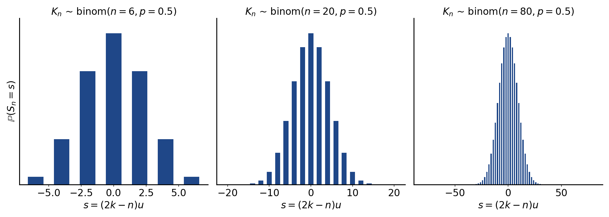
And another way to visualize this is to imagine larger and larger binomial trees (Figure $6$). The distribution for the locations $S_n$ for $n \in \{6, 20, 80\}$ are the distributions in Figure $5$.

Figure 6. As $n$ increases, the binomial tree expands, and the terminal distribution becomes wider and wider. More technically, the support increases as $K_n$'s binomial distribution's parameter $n$ increases.

To summarize so far, we have done something remarkable. We have modeled the motion of a completely random particle, and yet we can say something concrete and precise about its distribution of locations over time.

To do this, however, we had to assume that time was discrete. So the natural next question is: what’s the distribution of our process in the continuous-time limit? At this point in our story, it is not far-fetched to guess that it’s the normal distribution. De Moivre proved the De Moivre–Laplace theorem, the earliest version of a central limit theorem (CLT), in 1738, so roughly a hundred years before Robert Brown observed Brownian motion. So scientists and mathematicians already knew that a sum of independent and identically distributed random variables converge to a Gaussian. The key insight in the development of Brownian motion was to realize that the bombardment of a pollen particle could be modeled as such as a sum.

Convergence of a rescaled random walk

So now let’s imagine what happens when the molecular bombardments on our pollen particle increase in number but decrease proportionally in impact. So we have more bombardments but they move the pollen particle less per bombardment. This rescaling is critical, or else the variance of our process would explode. Put in physical terms, if we increased the number of bombardments of our pollen particle but did not scale down the size of the move, the pollen particle’s moves would grow implausibly large.

To formalize this, let’s first fix $p = 1/2$ so that $\mathbb{E}[Z_i] = 0$. We’ll handle the asymmetric case later. Now suppose that there are $n$ bombardments per unit of physical time $t$, so for any fixed amount of physical time $t \gt 0$, we can model the location of our pollen particle as

$B_t^{(n)} = u Z_1 + u Z_2 + \dots + u Z_{\lfloor tn \rfloor}, \quad u := \frac{1}{\sqrt{n}}. \tag{15}$

The notation ${\lfloor tn \rfloor}$ just indicates flooring to an integer since $t$ is a positive real number. And we need $u$ to scale with $n$, and so we set $u = 1 / \sqrt{n}$. If we take $n \rightarrow \infty$, then we get a continuous-time limit of a random walk:

$B_t = \lim_{n \rightarrow \infty} B_t^{(n)}. \tag{16}$

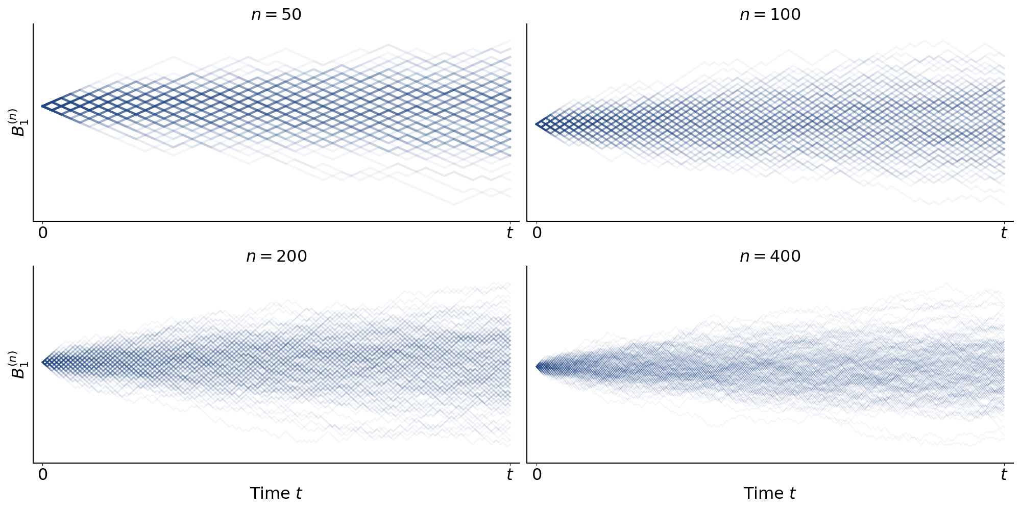
So again, we hold physical time $t$ fixed, and we make our binomial tree finer and finer (larger $n$ for fixed $t$). If we remove the grid of the binomial tree which clutters the visualization, and just visualize paths for finer and finer $n$, we can create visualizations similar to Figure $6$ but for much larger $n$ (Figure $7$).

Figure 7. Many simulations of binomial random walks with $p=1/2$ and increasing $n$. As $n$ increases, the size of the bombardment decreases. In the limit, we get a Brownian motion.

Now we can ask the same question we asked in the discrete-time case: after physical time $t$, what is the distribution of our pollen particle’s position? As we observed above, it must be a normal distribution! Here, the insight is not that the binomial distribution converges to the normal distribution—again, this was known a hundred years before Robert Brown’s observations. The insight is that by modeling the continuous-time limit of a random walk as in Equation $15$, this rescaled random walk $B_t^{(n)}$ converges to a normal distribution $\mathcal{N}(0, t)$.

Let’s see this a bit more formally. The De Moivre–Laplace theorem states that a properly standardized binomial random variable converges to the normal distribution. In our notation, $K_n \sim \text{binom}(n, p)$ with $p=1/2$, and the theorem states:

$\frac{K_n - \mathbb{E}[K_n]}{\sqrt{\mathbb{V}[K_n]}} = \frac{K_n - np}{\sqrt{npq}} = \frac{K_n - n/2}{\sqrt{n/4}} \;\stackrel{d}{\rightarrow}\; \mathcal{N}(0, 1). \tag{17}$

Now observe that $B_t^{(n)}$ is essentially this standardized quantity up to rescaling:

$\begin{aligned} B_t^{(n)} &= u Z_1 + u Z_2 + \dots + u Z_{\lfloor tn \rfloor} \\ &= \frac{1}{\sqrt{n}} \left( Z_1 + Z_2 + \dots + Z_{\lfloor tn \rfloor} \right) \\ &= \frac{1}{\sqrt{n}} \left(2 K_{\lfloor tn \rfloor} - {\lfloor tn \rfloor} \right) \\ &= \frac{1}{\sqrt{n}} \frac{\sqrt{\lfloor tn \rfloor}}{\sqrt{\lfloor tn \rfloor}} \; 2 \left(K_{\lfloor tn \rfloor} - {\lfloor tn \rfloor}/2 \right) \\ &= \sqrt{\frac{\lfloor tn \rfloor}{n}} \frac{K_{\lfloor tn \rfloor} - {\lfloor tn \rfloor}/2}{\sqrt{\lfloor tn \rfloor / 4}}. \end{aligned} \tag{18}$

By De Moivre–Laplace, we can say:

$\frac{K_{\lfloor tn \rfloor} - {\lfloor tn \rfloor}/2}{\sqrt{\lfloor tn \rfloor / 4}} \;\stackrel{d}{\rightarrow}\; \mathcal{N}(0, 1). \tag{19}$

And as $n \rightarrow \infty$, we can see that the prefactor converges to $\sqrt{t}$:

$\sqrt{\frac{\lfloor tn \rfloor}{n}} \;\rightarrow\; \sqrt{t}. \tag{20}$

Since the standardized binomial converges in distribution to $\mathcal{N}(0, 1)$ and the prefactor converges to the constant $\sqrt{t}$, we can see that

$B_t^{(n)} \;\stackrel{d}{\rightarrow}\; \sqrt{t} \; \mathcal{N}(0, 1) = \mathcal{N}(0, t). \tag{21}$

That’s it! As an aside, I think that in a modern treatment, we would invoke Slutsky’s theorem to arrive at Equation $21$. Slutsky’s theorem states that if a sequence of random variables converges in distribution and is multiplied by a sequence converging to a constant, then the product converges in distribution to the constant times the limit.

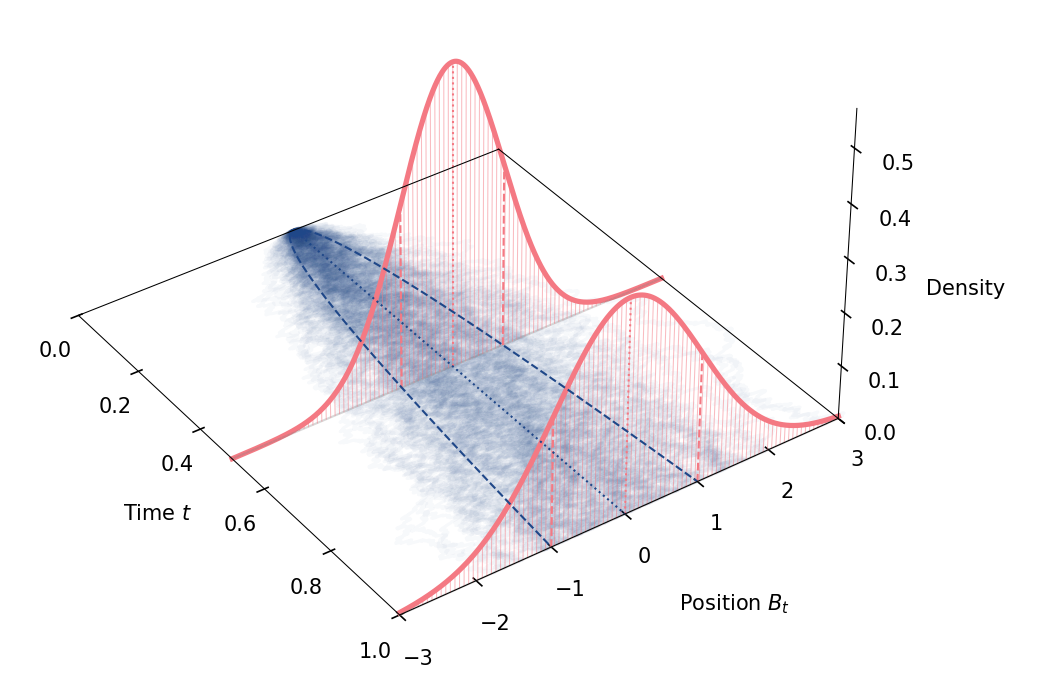
The geometric interpretation of this is that the marginal distribution after time $t$ is simply the normal distribution $\mathcal{N}(0, t)$ (Figure $8$).

Figure 8. The marginal distribution of a standard Brownian motion at time $t=0.5$ and $t=1$. In both cases, it is the normal distribution $\mathcal{N}(0, t)$. The mean (zero) and standard deviation ($\sqrt{t}$) are denoted with dashed lines.

Now that we see the simplest version of the derivation in its entirety, we can make two important adjustments. First, notice that our bombardment factor $u = 1/\sqrt{n}$ has no physical meaning. The denominator just ensures convergence, and so this bombardment has unit scale. But we can introduce a parameter $\sigma$ which captures the physical scale of the bombardment. Concretely, let

$u = \frac{\sigma}{\sqrt{n}}. \tag{22}$

It’s easy to see that this will flow through the derivation in Equation $18$ and give us

$\sigma B_t^{(n)} \;\stackrel{d}{\rightarrow}\; \sigma \sqrt{t} \; \mathcal{N}(0, 1) = \mathcal{N}(0, \sigma^2 t). \tag{23}$

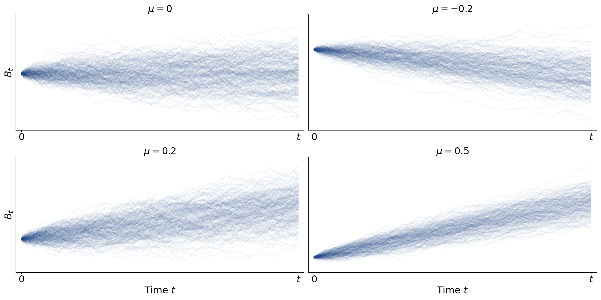
But I think the more interesting adjustment is adding a drift parameter $\mu$. Of course, we could just shift our Brownian motion directly:

$\mu + \sigma B_t^{(n)} \;\stackrel{d}{\rightarrow}\; \mathcal{N}(\mu, \sigma^2 t). \tag{24}$

But this has no physical meaning for our process. It’s just an arbitrary shift, not a drift. A richer way to approach this is to encode it directly into the bias of our coin flip. Intuitively, if we flip a biased coin (so $p \neq 1/2$), then the position our pollen particle will drift over time (Figure $9$).

Figure 9. Brownian motion with drift $\mu$.

However, there’s a problem with this approach: since $p$ is constrained to $[0, 1]$, then $\mathbb{E}[Z_i]$ is constrained to $[-1, 1]$, and thus the mean of our Brownian motion is constrained to $[-t, t]$:

$\begin{aligned} \mathbb{E}[Z_i] &= 2p - 1, \\ \mathbb{E}\!\left[B_t^{(n)}\right] &= \frac{1}{\sqrt{n}} \lfloor tn \rfloor \mathbb{E}[Z_1]. \end{aligned} \tag{25}$

A more elegant approach is to make $p$ a function $\mu$. However, we cannot naively do this, since our drift could explode as $n \rightarrow \infty$. So we need to normalize $\mu$ by $n$. Consider this definition for our bias parameter, now $p_n$:

$p_n = \frac{1}{2} + \frac{\mu}{2 \sigma \sqrt{n}}. \tag{26}$

Intuitively, the factor $\mu /(2 \sigma \sqrt{n})$ is the precise rate at which the bias of our coin has to vanish as we increase the number of bombardments $n$ per unit of physical time $t$. So the mean of each $Z_i$ is

$\mathbb{E}[Z_i] = 2 p_n - 1 = \frac{\mu}{\sigma \sqrt{n}}, \tag{27}$

and so the mean of our process—let’s denote it as $X_n^{(n)}$ since it is no longer standardized—converges to $\mu t$ as $n \rightarrow \infty$:

$\mathbb{E}\!\left[X_t^{(n)}\right] = \frac{\sigma}{\sqrt{n}} \lfloor tn \rfloor \mathbb{E}[Z_1] = \frac{\sigma}{\sqrt{n}} \lfloor tn \rfloor \frac{\mu}{\sigma \sqrt{n}} \;\rightarrow\; \mu t. \tag{28}$

Putting these two adjustments together—one for the drift and one for the size of the bombardment—we can see that the general result is non-standard Brownian motion:

$X_t^{(n)} \;\stackrel{d}{\rightarrow}\; \mathcal{N}(\mu t, \sigma^2 t). \tag{29}$

Alternatively, we could simply rewrite the main derivation (Equation $18$) using $u$ and $p_n$ as defined in Equations $22$ and $26$ respectively. This is arguably the more elegant derivation, since we construct the marginal distribution from the ground up. See A2 for this derivation.

Note that this isn’t a proof that the rescaled random walk converges to Brownian motion as a process. That requires more advanced mathematics such as Donsker’s theorem. Rather, it’s a claim about its marginal distribution at any fixed time $t$. But I think this provides amazing intuition for what Brownian motion really is without requiring much beyond elementary probability.

Conclusion

I still remember sitting in class for a course on probability and random process and watching the professor churn through the algebra to produce the insight in Equation $19$. It felt surprising and then obvious. The normal distribution is everywhere precisely because it is the limiting distribution for sums of independent and identically distributed random variables. We can shift or scale our random walk. We can make it asymmetric. It doesn’t really matter. We’ll still converge to a normal. And in my mind, this derivation builds good intuition for other properties of Brownian motion. For example, we can say that Brownian motion is a martingale or that it has stationary Gausian increments. The mathematics needed to make these claims precise might require some work, but the basic intuition is encoded in the derivations and visualizations above.

Appendix

A1. Binomial theorem

The binomial theorem is the following identity, which holds for any non-negative integer power $n$:

$(x + y)^n = \sum_{k=0}^n {n \choose k} x^k y^{n-k}. \tag{A1.1}$

This is easy to prove by induction. One can trivially check that the base case holds. And the inductive step is as follows:

$\begin{aligned} (x + y)^n (x + y) &= \sum_{k=0}^n {n \choose k} x^k y^{n-k} (x + y) \\ &= \sum_{k=0}^n {n \choose k} x^{k+1} y^{n-k} + \sum_{k=0}^n {n \choose k} x^k y^{n-k+1} \\ &:= A + B. \end{aligned} \tag{A1.2}$

If we write each sum $A$ and $B$ explicitly, it’s clear that we have $n-1$ overlapping terms:

$\begin{aligned} A &= {n \choose 0} x^1 y^n + {n \choose 1} x^2 y^{n-1} + \dots + {n \choose n-1} x^n y^1 + {n \choose n} x^{n+1} y^0, \\ \\ B &= {n \choose 0} x^0 y^{n+1} + {n \choose 1} x^1 y^n + \dots + {n \choose n-1} x^{n-1} y^2 + {n \choose n} x^n y^1. \end{aligned} \tag{A1.3}$

Collecting the $n-1$ like terms, we get:

$\begin{aligned} A+B &= \left[{n \choose 0} + {n \choose 1}\right] x^1 y^n + \dots + \left[{n \choose n-1} + {n \choose n}\right] x^n y^1 \\ &\quad + {n \choose 0} x^0 y^{n+1} + {n \choose n} x^{n+1} y^0. \end{aligned} \tag{A1.4}$

Finally, we can use the following identity to collapse bracketed binomial coefficients:

${n \choose k} = {n-1 \choose k-1} + {n-1 \choose k}. \tag{A1.5}$

And we can rewrite the non-overlapping terms in terms of $n+1$ since

${n \choose 0} = {n+1 \choose 0} = {n \choose n} = {n+1 \choose n+1} = 1. \tag{A1.6}$

This completes the inductive step:

$\begin{aligned} &(x+y)^{n+1} \\ &= {n+1 \choose 1} x^1 y^n + \dots + {n+1 \choose n} x^n y^1 + {n+1 \choose 0} x^0 y^{n+1} + {n+1 \choose n+1} x^{n+1} y^0 \\ &= \sum_{k=1}^{n+1} {n+1 \choose k} x^k y^{n+1-k}. \end{aligned} \tag{A1.7}$

Finally, the fact that the binomial distribution normalizes—discussed around Equation $8$—is simply a direct application of the binomial theorem for $x = p$ and $y=1-p$.

A2. Convergence with mean-centering and $\sigma$ scaling

Let $p_n$ be defined as

$p_n = \frac{1}{2} + \frac{\mu}{2 \sigma \sqrt{n}}. \tag{A3.1}$

Then clearly

$\begin{aligned} \mathbb{E}[Z_i] &= 2 p_n - 1 = \frac{\mu}{\sigma \sqrt{n}}, \\\\ \mu_{K} := \mathbb{E}[K_{\lfloor tn \rfloor}] &= {\lfloor tn \rfloor} p_n \\ &= {\lfloor tn \rfloor} \left( \frac{1}{2} + \frac{\mu}{2 \sigma \sqrt{n}}\right), \\\\ \sigma_{K}^2 := \mathbb{V}[K_{\lfloor tn \rfloor}] &= {\lfloor tn \rfloor} p_n (1 - p_n) \\ &= {\lfloor tn \rfloor} \left( \frac{1}{2} + \frac{\mu}{2 \sigma \sqrt{n}}\right) \left( \frac{1}{2} - \frac{\mu}{2 \sigma \sqrt{n}}\right) \\ &= {\lfloor tn \rfloor} \left( \frac{1}{4} - \frac{\mu^2}{4 \sigma^2 n}\right). \end{aligned} \tag{A3.2}$

Let’s redefine $X_t^{(n)}$ as the following sequence:

$X_t^{(n)} = u Z_1 + u Z_2 + \dots + u Z_{\lfloor tn \rfloor}, \quad u := \frac{\sigma}{\sqrt{n}}. \tag{A3.3}$

We can write this as:

$\begin{aligned} X_t^{(n)} &= \frac{\sigma}{\sqrt{n}} \left[ Z_1 + Z_2 + \dots + Z_{\lfloor tn \rfloor} \right] \\ &= \frac{\sigma}{\sqrt{n}} \left[ 2 K_{\lfloor tn \rfloor} - {\lfloor tn \rfloor} \right] \\ &= \frac{\sigma}{\sqrt{n}} \; 2 \left[ K_{\lfloor tn \rfloor} - \lfloor tn \rfloor \frac{1}{2} \right] \\ &= \frac{\sigma}{\sqrt{n}} \; 2 \left[ K_{\lfloor tn \rfloor} - \lfloor tn \rfloor \frac{1}{2} - {\lfloor tn \rfloor} \left( \frac{\mu}{2 \sigma \sqrt{n}}\right) + {\lfloor tn \rfloor} \left( \frac{\mu}{2 \sigma \sqrt{n}}\right) \right] \\ &= \frac{\sigma}{\sqrt{n}} \; 2 \left[ K_{\lfloor tn \rfloor} - \lfloor tn \rfloor \left( \frac{1}{2} - \frac{\mu}{2 \sigma \sqrt{n}} \right) \right] + {\lfloor tn \rfloor} \frac{\mu}{n} \\ &= \frac{\sigma}{\sqrt{n}} \; 2 \left[ K_{\lfloor tn \rfloor} - \mu_K \right] + {\lfloor tn \rfloor} \frac{\mu}{n} \\ &= \frac{\sigma}{\sqrt{n}} \sqrt{4 \frac{\lfloor tn \rfloor}{\lfloor tn \rfloor} \frac{1 - \frac{\mu}{\sigma^2 n}}{1 - \frac{\mu}{\sigma^2 n}}} \left[ K_{\lfloor tn \rfloor} - \mu_K \right] + {\lfloor tn \rfloor} \frac{\mu}{n} \\ &= \frac{\sigma}{\sqrt{n}} \sqrt{\lfloor tn \rfloor \left( 1 - \frac{\mu}{\sigma^2 n} \right)} \left[ \frac{K_{\lfloor tn \rfloor} - \mu_K}{\sqrt{\frac{\lfloor tn \rfloor \left(1 - \frac{\mu}{\sigma^2 n}\right)}{4}}} \right] + {\lfloor tn \rfloor} \frac{\mu}{n} \\ &= \frac{\sigma}{\sqrt{n}} \sqrt{\lfloor tn \rfloor \left( 1 - \frac{\mu}{\sigma^2 n} \right)} \left[ \frac{K_{\lfloor tn \rfloor} - \mu_K}{\sigma_K} \right] + {\lfloor tn \rfloor} \frac{\mu}{n} \end{aligned} \tag{A3.4}$

Finally, it’s clear that the prefactor converges to $\sigma \sqrt{t}$ as $n \rightarrow \infty$:

$\frac{\sigma}{\sqrt{n}} \sqrt{\lfloor tn \rfloor \left( 1 - \frac{\mu}{\sigma^2 n} \right)} \;\rightarrow\; \sigma \sqrt{t} \tag{A3.5}$

while the last term converges to $\mu t$ as $n \rightarrow \infty$:

${\lfloor tn \rfloor} \frac{\mu}{n} \;\rightarrow\; \mu t. \tag{A3.6}$

And since

$\frac{K_{\lfloor tn \rfloor} - \mu_K}{\sigma_K} \;\stackrel{d}{\rightarrow}\; \mathcal{N}(0, 1), \tag{A3.7}$

then again by Slutsky’s theorem, we know

$X_t^{(n)} \;\stackrel{d}{\rightarrow}\; \mathcal{N}(\mu t, \sigma^2 t). \tag{A3.8}$

So $X_t^{(n)}$ converges to a normal distribution with drift $\mu t$ and volatility $\sigma \sqrt{t}$.