Moving Averages

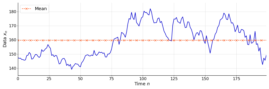
A moving average, sometimes called a rolling average, is a sequence of averages, constructed over subsets of a sequential data set. Moving averages are commonly used to process time series, particularly to smooth over noisy observations. For example, consider the noisy function in Figure $1$. If these data represents a time series, we may not be interested in a single point estimate of the mean (red dashed line). Instead, we may be interested in a sequence of mean estimates, constructed as the data becomes available. By having an average that “moves”, we could construct a new sequential data set that is a smoothed version of the input data.

Figure 1. A noisy function (blue solid line), along with the mean (red line, "x" markers) of the entire data set.

While moving averages are fairly simple conceptually, there are details that are useful to understand. In this post, I’ll discuss and implement the cumulative average, the simple moving average and the weighted moving average. I’ll also discuss a special case of the weighted moving average, the exponentially weighted moving average.

Cumulative average

Consider a sequential data set of $N$ observations,

$$\{x_1,x_2,\dots ,x_N\}.\text{\hspace{1em}(1)}$$

These data do not need to be a time series, but they do need to be ordered. For simplicity, I will refer to the index $n\in \{1,2,\dots ,N\}$ as “time”. Thus, at time $n$, the datum $x_n$ has just been observed, while the datum $x_{n+1}$ is the next observation. These are useful ways of talking about the problem setup, but the operations being discussed could be applied to any sequential data, such as a row of pixels in an image.

Perhaps the simplest way to make the point estimate in Figure $1$ “reactive” to new data is to compute a cumulative average (CA). In a CA, the sample mean is re-calculated as each new datum arrives. At time point $n$, the CA is defined as

$${\text{CA}}_n=\frac{x_1+x_2+\cdots +x_n}{n}.\text{\hspace{1em}(2)}$$

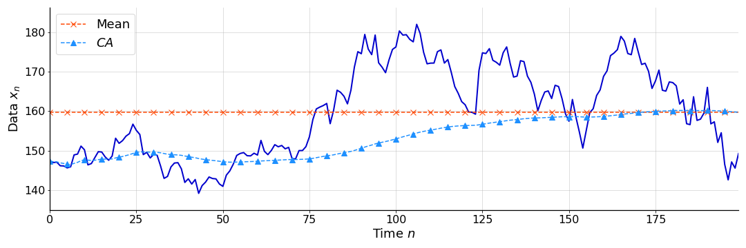
The effect is a sequence of mean estimates that account for increasingly more of the data. See Figure $2$ for an example of a simple CA applied to the data in Figure $1$. Clearly, at time point $N$, the mean of the entire data set (red dashed line) is equal to ${\text{CA}}_N$ (right-most point of blue dashed line).

Figure 2. The cumulative average (blue dashed line, "^" markers) computed on the function from Figure $1$.

We can implement a CA in Python as follows:

def ca(data):
    """Compute cumulative average over data.
    """
    return [mean(data[:i]) for i in range(1, len(data)+1)]

def mean(data):
    """Compute mean of data.
    """
    return sum(data) / len(data)

Notice, however, that re-computing the mean at each time point is inefficient. We could simply undo the normalization of the previous step, add the new datum, and then re-normalize. Formally, the relationship between ${\text{CA}}_n$ and ${\text{CA}}_{n+1}$ is

$${\text{CA}}_{n+1}=\frac{n\cdot {\text{CA}}_n+x_{n+1}}{n+1}.\text{\hspace{1em}(3)}$$

This results in a faster implementation:

def ca_iter(data):
    """Compute cumulative average over data.
    """
    m = data[0]
    out = [m]
    for i in range(1, len(data)):
        m = ((m * i) + data[i]) / (i+1)
        out.append(m)
    return out

As we’ll see, this idea of iteratively updating the mean, rather than fully recalculating it, is typical in moving average calculations.

Simple moving average

While the CA in Figure $2$ is certainly an improvement upon a single average in Figure $1$, we may want a sequence of estimates that are even more reactive. Look, for example, at the difference between the time series and the CA at $n=100$. The time series is rapidly increasing in value, but the CA is slow to react. One way to make the CA more reactive is to compute the average over a moving window of the data, where “window” refers to the subset of data in consideration. In other words, we can “forget” old data.

At each time point $n$, a simple moving average (SMA) computes the average over a backward-looking, fixed-width window. Let $K$ denote the window size. Then for each index $n$, we want to compute

$$\text{SMA}(K{)}_n=\frac{x_{n-k+1}+x_{n-k+2}+\cdots +x_{n-1}+x_n}{K}.\text{\hspace{1em}(4)}$$

Note that based on the definition in Equation $4$, the first $K-1$ elements in the sequence are ill-defined. We could define them in one of two ways:

$$\text{for }m<K,\text{SMA}(K{)}_m=\{\begin{array}{l}\text{undefined},\\ (x_1+x_2+\cdots +x_{m-1}+x_m)/m,\end{array}\text{\hspace{1em}(5)}$$

Following the convention used by Pandas, I’ll define $\text{SMA}(K{)}_m$ as undefined (or NaN).

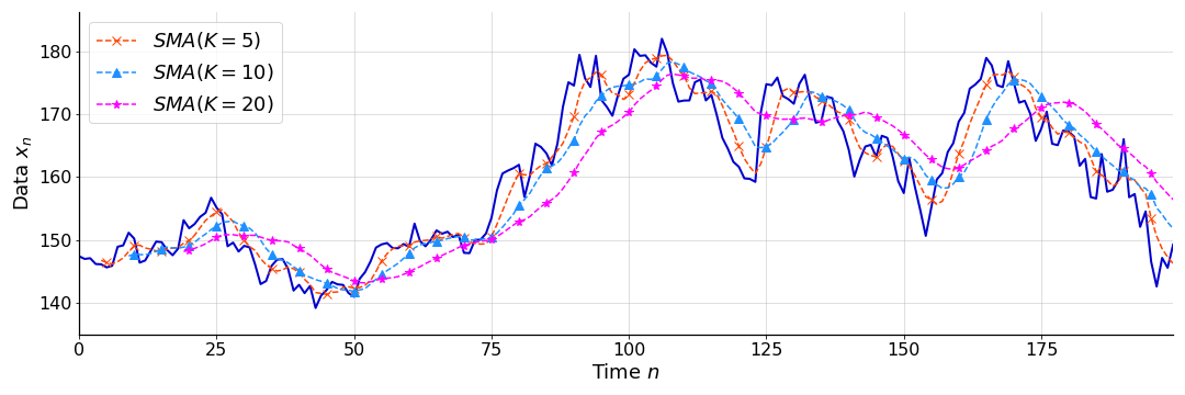
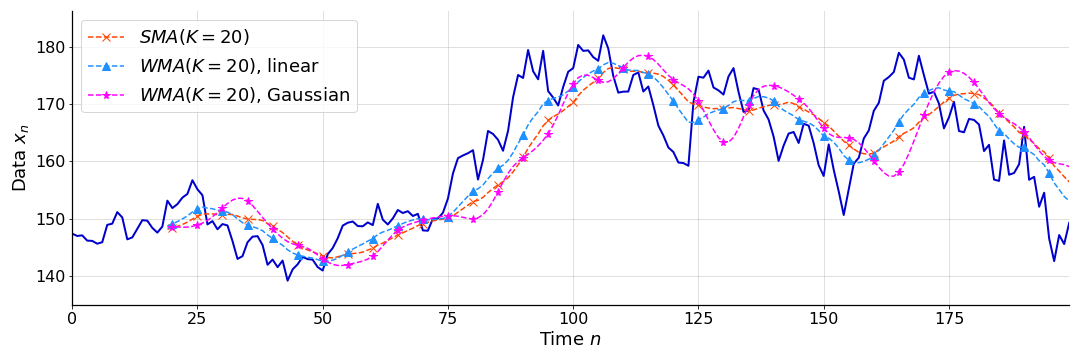
See Figure $3$ for an example of several SMAs with varying window sizes, applied to the noisy function in Figure $1$.

Figure 3. Three simple moving averages computed on the function from Figure $1$ (blue solid line). As the window size $K$ increases, the SMAs become smoother versions of the input function.

In Python, a simple moving average can be computed as follows:

nan = float('nan')

def sma(data, window):
    """Compute a simple moving average over a window of data.
    """
    out = [nan] * (window-1)
    for i in range(window, len(data)+1):
        m = mean(data[i-window:i])
        out.append(m)
    return out

However, there is a trick to computing SMAs even faster. Since the denominator never changes, we can update an existing mean estimate by subtracting out the datum that “falls” out of the window, and adding in the latest datum. This results in an iterative update rule,

$$\text{SMA}(K{)}_{n+1}=\text{SMA}(K{)}_n+\frac{x_{n+1}-x_{n-K+1}}{K}.\text{\hspace{1em}(6)}$$

In Python, this faster implementation is:

def sma_iter(data, window):
    """Iteratively compute simple moving average over window of data.
    """
    m = mean(data[:window])
    out = [nan] * (window-1) + [m]
    for i in range(window, len(data)):
        m += (data[i] - data[i-window]) / window
        out.append(m)
    return out

(Obviously, the code in this post is didactic, ignoring edge conditions like ill-defined windows.)

Weighted moving average

An obvious drawback of a simple moving average is that, if our sequential data changes abruptly, it may be slow to respond because it equally weights all the data points in the window. A natural extension would be to replace the mean calculation with a weighted mean calculation. This would allow us to assign relative importance to the observations in the window. This is the basic idea of a weighted moving average (WMA). Thus, each observation in the window has an associated weight,

$$\{w_1,w_2,\dots ,w_K\},\text{\hspace{1em}(7)}$$

and these are applied consistently (i.e. in the same order) as the window moves across the input. Formally, a weighted moving average is

$$\text{WMA}(K{)}_n=\frac{w_1{x}_{n-k+1}+w_2{x}_{n-k+2}+\cdots +w_{K-1}{x}_{n-1}+w_K{x}_n}{w_1+w_2+\cdots +w_K}.\text{\hspace{1em}(8)}$$

Note that this definition is agnostic to the specific weighting scheme used, and that the number of weights can grow with the number of observations ($K=n$ at each time point $n$).

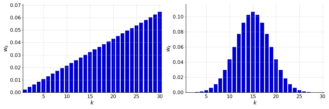
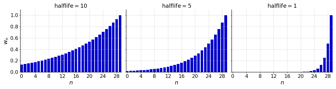
For example, we could use weights that emphasize the most recent datum, e.g. by decaying linearly with time ($w_k=k$), or we could use weights that smooth the data, e.g. by applying Gaussian distributed weights or a Gaussian filter ($w_k=\mathbb{P}(W=k)$ where $W$ is normally distributed). See Figure $4$ for examples of these weights.

Figure 4. Examples of weighting schemes that could be used in a weighted moving average. (Left) linearly decaying weights. (Right) Gaussian filter weights.

See Figure $5$ for a comparison of a simple moving average and a weighted moving average with both linearly decaying weights and Gaussian filter weights, both applied to the function in Figure $1$. We can see that the linearly decaying weights react more quickly to the signal than the SMA, and that the Gaussian weights smooth the function more.

Figure 5. A simple moving average (orange dashed line, "x" markers) compared with two weighted moving averages using linearly decaying weights (blue dashed line, "^" markers) and Gaussian distributed weights (pink dashed line, "*" markers).

In Python, a naive WMA can be implemented as follows:

def wmean(data, weights):
    """Compute weighted mean of data.
    """
    assert len(data) == len(weights)
    numer = [data[i] * weights[i] for i in range(len(data))]
    return sum(numer) / sum(weights)

def wma(data, weights):
    """Compute weighted moving average over data.
    """
    window = len(weights)
    out = [nan] * (window-1)
    for i in range(window, len(data)+1):
        m = wmean(data[i-window:i], weights)
        out.append(m)
    return out

I call this “naive” because it treats the weights as a moving window, which is an unnecessary constraint. As I mentioned above, the size of the window can grow with the number of observations. As with an SMA, there are tricks to computing WMAs even faster using iterative updates. However, the algorithmic details depend on the choice of weights. We’ll see one iterative update rule with exponentially decaying weights (below).

Exponential moving average

A poplar choice of WMA weights are ones that decay exponentially (Figure $6$). I have a couple ideas for why this choice is so common. First, much like linearly decaying weights (Figure $4$, left), exponentially decaying weights emphasize the most recent data points and can be chosen to decay approximately linearly near the current observation. However, exponentially decaying weights handle older data more elegantly: rather than a datum going from weighted to unweighted (or weight zero) when exiting the window, each datum is assigned a weight that decays asymptotically toward zero. In practice, we can stop tracking the weights once they are sufficiently close to zero. Secondly, exponentially decaying weights can be parameterized in a few ways, giving the modeler several ways to think about how the smoothing occurs.

Figure 6. Examples of exponentially decaying weights with varying halflives. As the halflife decreases, the weights decay more quickly.

As a reminder, let $y_0$ denote the initial quantity. Then the exponentially decaying function $y(x)$ can be expressed in the following parameterizations:

$$\begin{array}{r}y(x)=\{\begin{array}{ll}{y}_0{e}^{-\lambda x},& \text{decay parameter λ≥0},\\ y_0{\left(1/2\right)}^{x/h},& \text{halflife parameter h≥0},\\ y_0(1-\alpha {)}^x,& \text{decay rate α∈(0,1)}.\end{array}\end{array}\text{\hspace{1em}(9)}$$

See my previous post on exponential decay as needed. Note that in my previous post, I denoted the decay rate as $r$ rather than $\alpha$. Here, I’ve switched to $\alpha$ to match how I often see the parameter discussed in the context of EWMAs. Furthermore, $\alpha$ is sometimes called a smoothing factor rather than a decay rate, since changing $\alpha$ has the effect of smoothing (or not smoothing) the time series.

Given the various parameterizations, there are many ways we could implement EWMAs, and each parameterization lends itself to a different iterative updating scheme. Clearly, discussing each in turn would be too tedious. Thus, I’ll narrow the discussion in the following way: first, I’ll explain EWMA using the halflife parameterization, which is the most natural in my mind. I like halflives because they are in the natural units of the process (e.g. halflife in hours for data that is hourly). I won’t refine this much, though. Instead, I’ll switch to discussing EWMA using the rate parameterization (using $\alpha$), which is how I see often see it discussed (e.g. see Wikipedia and Pandas source code).

Halflife parameterization

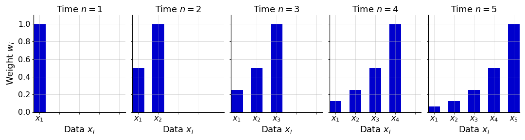
Recall that the halflife of exponential decay is the value in the domain at which the function reaches half of its initial value. Since exponential decay never reaches zero, the number of weights in an EWMA equals the number of observations so far ($K=n$). Thus, let’s think of the weight $w_i$ (where $i$ indexes the data up until time point $n$) as a function of the observation $x_i$. Using the halflife parameterization, the weight $w_i$ is defined as

$$w_i={\left(\frac{1}{2}\right)}^{(n-i)/h},i\in \{1,2,\dots ,n\}\text{\hspace{1em}(10)}$$

Obviously, this equation depends on my notation. If you assumed that $w_1$ was assigned to the most recent datum, Equation $10$ would be different. See Figure $7$ for an example of a sequence of exponentially decaying weights.

Figure 7. A sequence of exponentially decaying weights through time. At time $n=1$, there is a single weight. At time $n=2$, the single weight at time $n=1$ decays according to the halflife (here, $h=1$), while a new weight is introduced. And so on. For visualization purposes, the weights are normalized such that the newest weight is always equal to unity.

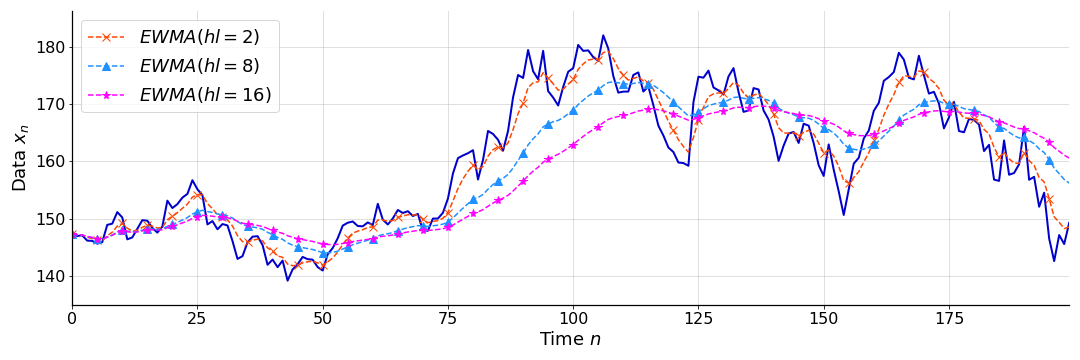
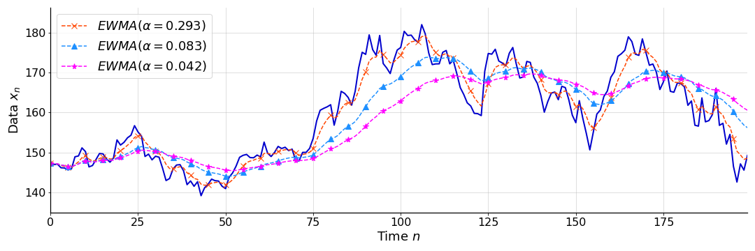
As I mentioned, in my mind, halflife is an intuitive parameter because it is in the natural units of the process. A shorter halflife means the EMA is more reactive to changes in data, while a longer halflife means that more historical data is considered for longer. So a bigger halflife means more smoothing. See Figure $7$ for a comparison of EWMAs with varying halflives, all applied to the function in Figure $1$.

Figure 8. Three exponentially weighted moving averages computed on the function from Figure $1$ (blue solid line). As the halflife increases, the EWMAs become smoother versions of the input function.

In Python, an EWMA can be implemented as follows:

def ewma_hl(data, halflife):
    """Compute exponentially weighted moving average with halflife over data.
    """
    weights = [(1/2)**(x/halflife) for x in range(len(data), 0, -1)]
    out = []
    for i in range(1, len(data)+1):
        m = wmean(data[:i], weights[:i])
        out.append(m)
    return out

Notice that I simply construct a set of exponentially decaying weights at the start, and then index into that set. This works for a subtle reason: since exponential decay is memoryless in the sense that the function decays as a fraction of its current quantity, the set of weights applied inside the weighted mean calculation (wmean) are always correct because they are normalized. If the un-normalized magnitude of the weights mattered, this implementation would not work.

Smoothing factor parameterization

Now let’s explore EWMAs in terms of the rate or smoothing factor $\alpha$. I think this parameterization is important if only because this is how many others think about and explain EWMAs. I’ll start by explaining what I’ll call the un-adjusted EWMA. This is an algorithm that approximates the exponentially decaying weights fairly well but is not technically correct, i.e. the weights do precisely exponentially decay. Then I’ll discuss the adjusted EWMA, which is simply the correct version of the un-adjusted approach. Why this terminology? I am simply borrowing from Pandas, which implements an EWMA with an adjust parameter.

To be clear, I’m not quite sure why the un-adjusted algorithm is discussed so often, since it technically incorrect and since both the halflife-parameterized algorithm and the adjusted EWMA are both easy to understand and correct. However, I’ve decided to discuss it simply since I have seen the un-adjusted formulation many times and never quite understood it. (When you see it, you should ask yourself why it is correct; in fact, it is not!)

Un-adjusted EWMA. A commonly discussed iterative update rule is the following,

$${\text{EWMA}}_n=\{\begin{array}{ll}{x}_1,& \text{n=1},\\ \alpha x_n+(1-\alpha )\cdot {\text{EWMA}}_{n-1},& \text{n>1,α∈(0,1)}.\end{array}\text{\hspace{1em}(11)}$$

Wikipedia cites the National Institute of Standards and Technology website, which in turn cites (Hunter, 1986) for this rule. We’ll investigate what Equation $11$ means and why it works in a moment. For now, let’s assume it is correct and just think about how to interpret it. (Hunter, 1986) has an interesting perspective. Let’s think of ${\text{EWMA}}_n$ as the predicted value of the time series at time $n$. Let’s denote this ${\hat{x}}_{n+1}$. Thus,

$${\text{EWMA}}_n={\hat{x}}_{n+1}.\text{\hspace{1em}(12)}$$

Now let’s rewrite the update rule in Equation $11$ as

$$\begin{array}{rl}{\hat{x}}_{n+1}& =\alpha x_n+(1-\alpha ){\hat{x}}_n,\\ & \Downarrow \\ {\hat{x}}_{n+1}& ={\hat{x}}_n+\alpha (x_n-{\hat{x}}_n).\end{array}\text{\hspace{1em}(13)}$$

In other words, the next predicted value in the time series is the current predicted value in the time series, plus some fraction of the error between what we observed and what we predicted. If $\alpha =1$, then we would not believe our predictive model at all. The next predicted value would be the current observation. This EWMA would simply reconstruct the original time series. (Hence why $\alpha <1$ is a restriction.) If $\alpha =0$, then we would not trust our observations at all. The next predicted value would always be the initial value $x_1$. (Hence why $\alpha >0$ is a restriction.) Alternatively, we can think of the next prediction as a convex combination of the current observation and the current prediction.

Either way, to quote (Hunter, 1986), $\alpha$ “determines the depth of memory of the EWMA”. See Figure $9$ for examples of EWMAs with $\alpha$ parameters chosen to match the halflives in Figure $8$. At the end, I’ll discuss this reparameterization from $\alpha$ to $h$.

Figure 9. Three exponentially weighted moving averages computed on the function from Figure $1$ (blue solid line) using the smoothing factor $\alpha$. The $\alpha$ values were chosen to match the halflives in Figure $9$. See Equation $23$ for details.

Now that we have some intuition for this formulation, let’s ask ourselves the obvious question: how does Equation $11$ (or $13$) model a moving average with exponentially decaying weights? Let’s write down the formula for the first few data points:

$$\begin{array}{rl}{\hat{x}}_2& =x_1,\\ & \\ {\hat{x}}_3& =\alpha x_2+(1-\alpha ){\hat{x}}_2\\ & =\alpha x_2+(1-\alpha )x_1\\ & \\ {\hat{x}}_4& =\alpha x_3+(1-\alpha ){\hat{x}}_3\\ & =\alpha x_3+(1-\alpha )[\alpha x_2+(1-\alpha )x_1]\\ & =\alpha x_3+\alpha (1-\alpha )x_2+(1-\alpha {)}^2{x}_1\\ & ⋮\end{array}\text{\hspace{1em}(14)}$$

Note that we can distribute the $\alpha$ and generalize this to

$$\begin{array}{rl}{\hat{x}}_{n+1}& =\alpha \left[x_n+(1-\alpha )x_{n-1}+(1-\alpha {)}^2{x}_{n-2}+\cdots +(1-\alpha {)}^{n-2}{x}_2\right]\\ & +(1-\alpha {)}^{n-1}{x}_1.\end{array}\text{\hspace{1em}(15)}$$

Here, we can see why Equation $13$ approximates a weighted moving average with exponentially decaying weights. With the exception of the weight associated with the first datum $x_1$, the $k$-th weight is defined as

$$w_k=\alpha (1-\alpha {)}^{n-k}.\text{\hspace{1em}(16)}$$

Note that we are computing the weighted mean on the fly, meaning that these weights must sum to unity. Using basic properties of geometric series, we can verify this:

$$\begin{array}{rl}\alpha \sum _{i=0}^{n-2}(1-\alpha {)}^i+(1-\alpha {)}^{n-1}& =\alpha \left[\frac{1-(1-\alpha {)}^{n-1}}{1-(1-\alpha )}\right]+(1-\alpha {)}^{n-1}\\ & =1-(1-\alpha {)}^{n-1}+(1-\alpha {)}^{n-1}\\ & =1.\end{array}\text{\hspace{1em}(17)}$$

So this approach is reasonable. However, the weight associated with the first datum is incorrect. It should be $\alpha (1-\alpha {)}^{n-1}$, yet it is only $(1-\alpha {)}^{n-1}$. For sufficiently large $n$, this term should be close to zero. While the error is typically quite small, there is an error. An “adjusted” EWMA (discussed next) is simply the correct formulation. As I mentioned, it’s useful to understand the un-adjusted approach, because it comes up often, but in practice, I think there’s no reason not to just understand and use the adjusted approach.

Adjusted EWMA. The correct update rule is the following:

$${\hat{x}}_{n+1}=\frac{x_n+(1-\alpha )x_{n-1}+(1-\alpha {)}^2{x}_{n-2}+\cdots +(1-\alpha {)}^{n-1}{x}_1}{1+(1-\alpha )+(1-\alpha {)}^2+...+(1-\alpha {)}^{n-1}}.\text{\hspace{1em}(18)}$$

Here, we update each datum with the weight

$$w_k=(1-\alpha {)}^{n-k}.\text{\hspace{1em}(19)}$$

And we normalize the calculation at each time point by dividing by the sum of the weights. It’s pretty easy to see that both the numerator and denominator in Equation $18$ can be updated recursively:

$$\begin{array}{rl}{\text{numer}}_n& =x_n+(1-\alpha )\cdot {\text{numer}}_{n-1},\\ {\text{denom}}_n& =1+(1-\alpha )\cdot {\text{denom}}_{n-1}.\end{array}\text{\hspace{1em}(20)}$$

This gives us a fast, iterative algorithm to exactly compute an EWMA online. In my mind, Equation $20$ is very simple to reason about and implement.

In Python, an EWMA with smoothing factor $\alpha$ can be computed as follows:

def ewma_alpha(data, alpha):
    num = data[0]
    den = 1
    out = [num/den]
    for i in range(1, len(data)):
        num = data[i] + (1 - alpha) * num
        den = 1 + (1 - alpha) * den
        out.append(num/den)
    return out

This is the code that is used to produce Figure $9$.

Switching parameterizations

As a final comment, it’s useful to be able to switch to between the halflife and smoothing parameterizations. In my post on exponential decay, I showed that the smoothing factor $\alpha$ is related to the decay parameter $\lambda$ in the following way:

$$\lambda =-\ln (1-\alpha ).\text{\hspace{1em}(21)}$$

Later in the post, I also showed that halflife is related to decay in the following way:

$$h=\frac{\ln (2)}{\lambda }.\text{\hspace{1em}(22)}$$

Using these two equations, we can easily solve for $\alpha$ in terms of $h$ or vice versa:

$$\begin{array}{rl}\alpha & =1-2^{-1/h},\\ h& =\frac{1}{-{\log }_2(1-\alpha )}.\end{array}\text{\hspace{1em}(23)}$$

These operations are useful when you want to work in a particular parameterization that is not supported by a given EWMA implementation.