OLS with Heteroscedasticity

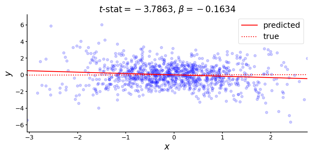
Consider this linear relationship with true coefficient $\beta =0.01$ and no intercept (Figure $1$):

from numpy.random import RandomState

rng   = RandomState(seed=0)
x     = rng.randn(1000)
beta  = 0.01
noise = rng.randn(1000) + x*rng.randn(1000)
y     = beta * x + noise

Let’s fit ordinary least squares (OLS) to these data and look at the estimated $\hat{\beta }$ and $t$-statistic:

import statsmodels.api as sm

ols = sm.OLS(y, x).fit()
print(f'{ols.params[0]:.4f}')   # beta  : -0.1634
print(f'{ols.tvalues[0]:.4f}')  # t-stat: -3.7863

Remarkably, we see that the sign of the coefficient is wrong, yet the $t$-statistic is large in magnitude. Assuming normally distributed error terms, a $t$-statistic of $-3.78$ indicates that our estimated coefficient, $\hat{\beta }=-0.1634$, is nearly four standard deviations from the null hypothesis (here, zero). (See my previous post on hypothesis testing for OLS if this claim does not make sense.) This is obviously wrong, but what’s going on here? The problem is in the noise term:

noise = rng.randn(1000) + x*rng.randn(1000)

Each element in the vector noise is a function of its corresponding element in x. This breaks an assumption in OLS and results in incorrectly computed $t$-statistics. The goal of this post is to look at this phenomenon (heteroscedasticity) and some solutions in general.

Figure 1. OLS fit to data with heteroscedastic errors. The sign of the coefficient is wrong, yet the model has estimated a large $t$-statistic due to heteroscedasticity which is unaccounted for.

Non-spherical errors

Recall the OLS model,

$$\mathbf{y}=\mathbf{X}\mathbf{\beta }+\mathbf{\epsilon },\text{\hspace{1em}(1)}$$

where $\mathbf{y}$ is an $N$-vector of response variables, $\mathbf{X}$ is an $N\times P$ matrix of $P$-dimensional predictors, $\mathbf{\beta }$ specifies a $P$-dimensional hyperplane, and $\mathbf{\epsilon }$ is an $N$-vector of noise terms. We could include an intercept by adding a column of ones to $\mathbf{X}$. A standard assumption of OLS is spherical errors (see Assumption $4$ here). Formally, spherical errors assumes

$$\mathbb{V}[\mathbf{\epsilon }\mid \mathbf{X}]={\sigma }^2\mathbf{I}.\text{\hspace{1em}(2)}$$

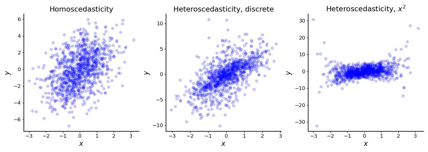
In words, all noise terms ${\mathbf{\epsilon }}_n$ for $n\in \{1,\dots ,N\}$ share a constant variance (Figure $2$, left). This assumption may be reasonable when our data are approximately i.i.d., but this is often not the case. Let’s look at the simple scenario in which this assumption does not hold: when the error terms are heteroscedastic.

In statistics, scedasticity refers to the distribution of the error terms. OLS assumes homoscedasticity, which means that each sample’s error term has a constant variance (${\sigma }^2$ in Equation $2$). With heterscedasticity, each sample ${\mathbf{x}}_n$ has an error term with its own variance. Formally, Equation $2$ becomes

$$\mathbb{V}[\mathbf{\epsilon }\mid \mathbf{X}]=\left[\begin{array}{cccc}{\sigma }_1^2& 0& \dots & 0\\ 0& {\sigma }_2^2& \dots & 0\\ ⋮& ⋮& \ddots & ⋮\\ 0& 0& \dots & {\sigma }_N^2\end{array}\right].\text{\hspace{1em}(3)}$$

There are multiple forms of heteroscedasticity. Consider, for example, data which can be partitioned into distinct groups. These types of data may exhibit discrete heteroscedasticity, since each group may have its own variance (Figure $2$, middle). A real-world instance of discrete heteroscedasticity might arise when data is collected from multiple sources, such as if each city or province in a country is responsible for reporting its own census data.

Alternatively, consider data in which each datum’s variance depends on a single predictor. These data may exhibit heteroscedasticity along that dimension (Figure $2$, right). For example, in time series data, variance might change over time. This type of heteroscedasticity was the source of our problems in the leading example.

Figure 2. Data exhibiting homoscedasticity (left), discrete heteroscedasticity (middle), and heteroscedasticity of the form ${\epsilon }_n\sim \mathcal{N}(0,x_n^2)$.

A second challenge for OLS is when the error terms are correlated, inducing autocorrelation in the observations. Then Equation $3$ becomes

$$\mathbb{V}[\mathbf{\epsilon }\mid \mathbf{X}]=\left[\begin{array}{cccc}{\sigma }^2& {\rho }_{12}& \dots & {\rho }_{1N}\\ {\rho }_{21}& {\sigma }^2& \dots & {\rho }_{2N}\\ ⋮& ⋮& \ddots & ⋮\\ {\rho }_{N1}& {\rho }_{N2}& \dots & {\sigma }^2\end{array}\right].\text{\hspace{1em}(4)}$$

We could, of course, have both heteroscedasticity and autocorrelation, in which case the diagonal in Equation $4$ would be replaced with the diagonal in Equation $3$. In this post, I will limit the discussion to only the first scenario, heteroscedastic errors.

Incorrect estimation with OLS

So what happens when we apply classic OLS to data with variance

$$\mathbb{V}[\mathbf{\epsilon }\mid \mathbf{X}]={\sigma }^2\mathbf{\Omega },\text{\hspace{1em}(5)}$$

instead of spherical errors. Here, $\mathbf{\Omega }$ is a positive definite matrix that allows for heteroscedasticity or autocorrelation. First, observe that the estimator from classic OLS,

$$\hat{\mathbf{\beta }}=({\mathbf{X}}^{\top }\mathbf{X}{)}^{-1}{\mathbf{X}}^{\top }\mathbf{y}\text{\hspace{1em}(6)}$$

is still unbiased, even with a generalized noise term:

$$\begin{array}{rl}\mathbb{E}[\hat{\mathbf{\beta }}\mid \mathbf{X}]& =\mathbb{E}[({\mathbf{X}}^{\top }\mathbf{X}{)}^{-1}{\mathbf{X}}^{\top }\mathbf{y}\mid \mathbf{X}]\\ & =({\mathbf{X}}^{\top }\mathbf{X}{)}^{-1}{\mathbf{X}}^{\top }\mathbb{E}[\mathbf{y}\mid \mathbf{X}]\\ & =({\mathbf{X}}^{\top }\mathbf{X}{)}^{-1}{\mathbf{X}}^{\top }\mathbf{X}\mathbf{\beta }\\ & =\mathbf{\beta }\end{array}\text{\hspace{1em}(7)}$$

This holds because we still assume that $\mathbb{E}[\mathbf{\epsilon }\mid \mathbf{X}]=0$, if we still assume that while the errors can be heteroscedastic, their conditional expectation is still zero.

However, despite still being unbiased, the OLS estimator still has a problem. Deriving the OLS variance,

$$\mathbb{V}[\hat{\mathbf{\beta }}\mid \mathbf{X}]={\sigma }^2({\mathbf{X}}^{\top }\mathbf{X}{)}^{-1}.\text{\hspace{1em}(8)}$$

requires assuming homoscedasticity (see Equation $10$ here). Without this assumption, the correct variance would be

$$\mathbb{V}[\hat{\mathbf{\beta }}\mid \mathbf{X}]={\sigma }^2({\mathbf{X}}^{\top }\mathbf{X}{)}^{-1}{\mathbf{X}}^{\top }\mathbf{\Omega }\mathbf{X}({\mathbf{X}}^{\top }\mathbf{X}{)}^{-1}.\text{\hspace{1em}(9)}$$

This follows immediately from plugging in $\mathbb{V}[\mathbf{\epsilon }\mid \mathbf{X}]={\sigma }^2\mathbf{\Omega }$ into Equation $10$ in the previous post, and we cannot simplify it further without assuming some structure for the error terms.

The second problem is that $s^2$ is no longer an unbiased estimate of ${\sigma }^2$. Logically, this holds since there is no longer a single ${\sigma }^2$. Furthermore, the derivation for the unbiasedness of $s^2$ depends on homoscedasticity. (See Equation $22$ here.)

We can now see that this is why we estimated incorrect $t$-statistics in the leading example. Recall that the $t$-statistic for the $p$-th coefficient of $\hat{\mathbf{\beta }}$ is

$$t_p=\frac{{\hat{\beta }}_p-b_p}{\sqrt{s^2{\left[({\mathbf{X}}^{\top }\mathbf{X}{)}^{-1}\right]}_{pp}}}\text{\hspace{1em}(10)}$$

where $b_p$ is the hypothesized true value and the denominator is the standard error. (See my previous post for details.) Both the estimated variance and $s^2$ are incorrect without homoscedasticity being true. In fact, it’s impossible to know if the $t$-statistic will be too large, too small, or correct without knowing more about ${\sigma }^2\mathbf{\Omega }$.

Asymptotic behavior

Finally, let’s consider the asymptotic behavior of the OLS estimator. A standard assumption is that

$$\mathrm{plim}\frac{1}{N}{\mathbf{X}}^{\top }\mathbf{X}=\mathbf{Q},\text{\hspace{1em}(11)}$$

for some positive definite matrix $\mathbf{Q}$. This is a reasonable assumption because of the weak law of large numbers. The basic idea is that our data are “well-behaved” in the sense that they converge to their expected values. (See this post on OLS consistency for discussion.)

However, notice that ${\mathbf{X}}^{\top }\mathbf{\Omega }\mathbf{X}$ (the middle term in Equation $9$) is more subtle. Without knowing anything about $\mathbf{\Omega }$, there is no guarantee that ${\mathbf{X}}^{\top }\mathbf{\Omega }\mathbf{X}$ will converge in probability to some matrix. However, even if we did assume this, that

$$\mathrm{plim}\frac{1}{N}{\mathbf{X}}^{\top }\mathbf{\Omega }\mathbf{X}=\mathbf{C}\text{\hspace{1em}(12)}$$

for some matrix $\mathbf{C}$, then all we could say is that the OLS estimator converges in distribution to

$$\sqrt{N}(\hat{\mathbf{\beta }}-\mathbf{\beta })\stackrel{d}{\to }\mathcal{N}(0,{\sigma }^2{\mathbf{Q}}^{-1}\mathbf{C}\mathbf{Q}).\text{\hspace{1em}(13)}$$

But we cannot simplify the covariance matrix, and $\mathrm{plim}{s}^2\ne {\sigma }^2$.

Summary

In short, without homoscedasticity, the nice properties of the OLS estimator do not hold, and inference using OLS on heteroscedastic data will be incorrect. There are a few solutions to this problem. The first is to use generalized least squares (GLS) if we do know the variance. This is because GLS is the best linear unbiased estimator when assuming generalized error terms. Another approach is to still use OLS but to use heteroscedasticity-robust standard errors instead of the usual standard errors. Finally, in some situations, we can use weighted least squares. I will discuss these topics in more detail in future posts.