Bayesian Online Changepoint Detection

Introduction

Given sequential data such as stock market prices or streaming stories in a newswire, we might be interested in when these data change in some way, such as a stock price falling or the document topics shifting. If we view our data as observations from a generative process, then we care about when the generative parameters change. An abrupt change in these parameters is called a changepoint, and changepoint detection is the modeling and inferring of these events.

The goal of this post is to explain Ryan P. Adams and David J.C. MacKay’s technical report on Bayesian online changepoint detection (Adams & MacKay, 2007) in my own words, and to work through the framework and code for a particular model. While I focus my discussion on Adams and MacKay’s paper, (Fearnhead & Liu, 2007) is a similar model for the same problem, and it is worth reading as a comparison.

Understanding this post will require understanding conjugacy and the exponential family. The example implementation requires understanding Bayesian inference for the Gaussian.

Model

Let $x_t\in {\mathbb{R}}^d$ denote the $t$-th observation in a data sequence, and let ${\mathbf{x}}_{s:t}$ denote the sequence $x_s,x_{s+1},\dots ,x_{t-1},x_t$ for $s\le t$. We assume that our $T$ data points ${\mathbf{x}}_{1:T}$ can be partitioned such that the data within each partition are i.i.d. samples from some distribution; this is the product partition model (Barry & Hartigan, 1992). Formally, let ${\mathbf{\theta }}^{(p)}$ denote the generative parameters for partition $p$ and ${\mathbf{\theta }}_0$ denote the hyperprior. Then ${\mathbf{\theta }}^{(p)}\sim p({\mathbf{\theta }}_0)$ are i.i.d. for partitions $p=1,2,\dots ,P$ (Figure $1\text{a}$).

Figure 1. Conceptual diagrams of (a) synthetic data partitioned by two changepoints—the changepoint for the third partition is unknown—and (b) the associated run length $r_t$ as a function of time $t$. Changepoints occur between partitions, and $r_t$ drops to $0$ at a changepoint.

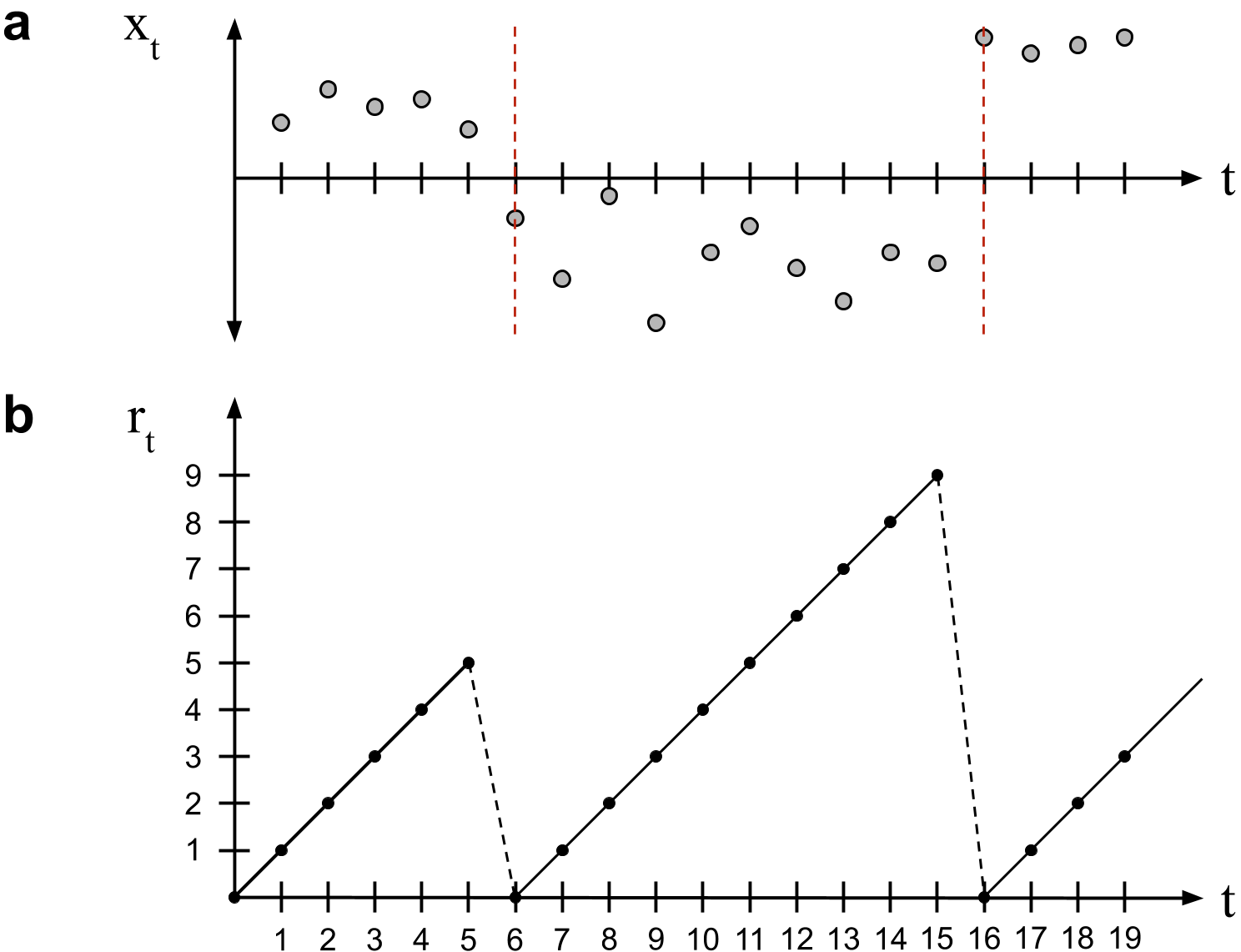
Bayesian online changepoint detection works by modeling the time since the last changepoint, called the run length. The run length at time $t$ is denoted $r_t$. Logically, it can take one of two values,

$$r_t=\{\begin{array}{ll}0& \text{if changepoint at time t}\\ r_{t-1}+1& \text{else}.\end{array}$$

In words, the run length only ever increases by one or drops to zero (Figure $1\text{b}$). The transition probabilities are modeled by the changepoint prior $p(r_t\mid r_{t-1})$, which is the assumption that $r_t$ is conditionally independent of everything else given $r_{t-1}$.

Ultimately, we want to infer both the run-length posterior distribution $p(r_t\mid {\mathbf{x}}_{1:t})$ and the posterior predictive distribution $p(x_{t+1}\mid {\mathbf{x}}_{1:t})$ so that we can predict the next data point given all the data we have seen so far.

Recursive RL posterior estimation

In Bayesian inference, if $\mathcal{D}$ is a set of $N$ i.i.d. observations $\{{\mathbf{x}}_n{\}}_{n=1}^N$ and $\mathbf{\theta }$ are model parameters, then the posterior predictive distribution over a new observation $\hat{\mathbf{x}}$ is

$$p(\hat{\mathbf{x}}\mid \mathcal{D})=\int \stackrel{\text{Model}}{\overbrace{p(\hat{\mathbf{x}}\mid \mathbf{\theta })}}\stackrel{\text{Posterior}}{\overbrace{p(\mathbf{\theta }\mid \mathcal{D})}}\text{d}\mathbf{\theta }.$$

In words, we weigh our probabilistic model’s predictions by our posterior uncertainty of the model’s parameters. Marginalization means doing this for every possible parameter value. In Bayesian online changepoint detection, this posterior takes a slightly different form. The posterior predictive is the probability of the next data point, $x_{t+1}$, given the observations so far, ${\mathbf{x}}_{1:t}$, and it is computed by marginalizing out the run length $r_t$,

$$\begin{array}{rl}p(x_{t+1}\mid {\mathbf{x}}_{1:t})& =\sum _{r_t}p(x_{t+1},r_t\mid {\mathbf{x}}_{1:t})\\ & =\sum _{r_t}\stackrel{\text{UPM predictive}}{\overbrace{p(x_{t+1}\mid r_t,{\mathbf{x}}^{(\ell )})}}\stackrel{\text{RL posterior}}{\overbrace{p(r_t\mid {\mathbf{x}}_{1:t})}}.\end{array}\text{\hspace{1em}(1)}$$

We use ${\mathbf{x}}^{(\ell )}$ to denote all observations associated with $r_t=\ell$. If this is confusing, think of $r_t=\ell$ as a hypothesis that a changepoint occurred $\ell$ time steps ago. Thus, only data within the past $\ell$ time points should contribute to our predictive distribution over ${\mathbf{x}}_{t+1}$. This notation is a little sloppy, and we could write equation $1$ more explicitly as

$$p(x_{t+1}\mid {\mathbf{x}}_{1:t})=\sum _{\ell =0}^{t}p(x_{t+1}\mid r_t=\ell ,{\mathbf{x}}_{(t-\ell ):t})p(r_t=\ell \mid {\mathbf{x}}_{1:t}).$$

While Adams and MacKay refer to the term analogous to “model” as a “marginal predictive”, I will use underlying probabilistic model (UPM) predictive to clearly disambiguate it from other predictives in this discussion. In the next section, we will see how to efficiently compute this term. For now assume that it is straightforward.

If we can compute the UPM predictive, then we just need to compute the RL posterior, which is proportional to the joint,

$$p(r_t\mid {\mathbf{x}}_{1:t})=\frac{p(r_t,{\mathbf{x}}_{1:t})}{{\sum }_{r_{t^{\prime }}}p(r_{t^{\prime }},{\mathbf{x}}_{1:t})}.\text{\hspace{1em}(2)}$$

We can write this joint recursively as

$$\begin{array}{rl}p(r_t,{\mathbf{x}}_{1:t})& =\sum _{r_{t-1}}p(r_t,r_{t-1},x_t,{\mathbf{x}}_{1:t-1})\\ & =\sum _{r_{t-1}}p(r_t,x_t\mid r_{t-1},{\mathbf{x}}_{1:t-1})p(r_{t-1},{\mathbf{x}}_{1:t-1})\\ & =\sum _{r_{t-1}}p(x_t\mid r_t,\cancel{r_{t-1}},{\mathbf{x}}^{(\ell )})p(r_t\mid r_{t-1},\cancel{{\mathbf{x}}_{1:t-1}})p(r_{t-1},{\mathbf{x}}_{1:t-1})\end{array}$$

The first two steps are just marginalization and the chain rule. However, the third step is trickier because it only holds if our modeling assumptions are made. Both of these equations

$$\begin{array}{rl}p(r_t\mid r_{t-1},{\mathbf{x}}_{1:t-1})& =p(r_t\mid r_{t-1}),\\ p(x_t\mid r_t,r_{t-1},{\mathbf{x}}_{1:t-1})& =p(x_t\mid r_t,{\mathbf{x}}^{(\ell )})\end{array}$$

fall out of our modeling assumptions. Summarizing and annotating the derivation, we have

$$p(r_t,{\mathbf{x}}_{1:t})=\sum _{r_{t-1}}\stackrel{\text{UPM predictive}}{\overbrace{p(x_t\mid r_t,{\mathbf{x}}^{(\ell )})}}\stackrel{\text{Changepoint prior}}{\overbrace{p(r_t\mid r_{t-1})}}\stackrel{\text{Message}}{\overbrace{p(r_{t-1},{\mathbf{x}}_{1:t-1})}}.\text{\hspace{1em}(3)}$$

We now have a recursive algorithm for computing the RL posterior. The algorithm is recursive because after we compute the joint distribution $p(r_{t-1},{\mathbf{x}}_{1:t-1})$, we can forward message-pass this distribution’s mass to the calculation for $p(r_t,{\mathbf{x}}_{1:t})$. Of course, a recursive algorithm must define its initial conditions (what is $p(r_0)$?), and we will address this later.

As an aside, when I first read the paper, Equation $3$ seemed as if it arose ex nihilo. In my mind, the authors dreamed up $r_t$, knew to marginalize out $r_{t-1}$, and voilà! a recursive algorithm. In fact, Equation $3$ is similar to the forward algorithm for hidden Markov models. In this context, $r_t$ is the latent variable, and there are no generative parameters. Wikipedia’s derivation is quite clear; for stable reference, consult either (Bishop, 2006) or (Murphy, 2012).

It is useful to think about this recursive algorithm visually. Borrowing language from the paper, we can visualize the message-passing algorithm as living on a trellis (Figure $2$). At each time point, mass is either passed “upward” such that the run-length is incremented or “downward” where it is truncated to zero. At each time point $t$, the discrete RL posterior distribution has support over $t+1$ values.

Figure 2. Diagram of the message-passing algorithm. Each node has associated mass. For example, the probability of $p(r_4=2,{\mathbf{x}}_{1:4})$ is associated with the node indexed by $t=4$ and $r_t=2$.

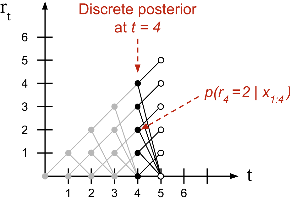
This observation has an important algorithmic consequence. When we compute what Adams and MacKay call the growth probabilities or the probability that the run-length increases, the summation in Equation $3$ disappears because each term in the summation is zero except when $r_t=r_{t-1}+1$. It is only when calculating the changepoint probabilities, when the mass is passed downwards, that we sum over previous joint probabilities.

In summary, provided we can compute the UPM predictive and the changepoint prior in Equation $3$ and can initialize our recursive algorithm, we will have everything we need for both inference and prediction. Let’s tackle these in that order.

Underlying probabilistic model

Computing the UPM predictive leverages conjugacy and the exponential family. In principle, one could abbreviate this section as most of it is not methodologically novel to the paper. However, when I first read the paper, computing the UPM predictive was not obvious to me, and I will go into detail to explain it.

We assume our model is from an exponential family (EF) member with parameters $\mathbf{\eta }$. To compute $p(x_{t+1}\mid r_t=\ell ,{\mathbf{x}}^{(\ell )})$, we could integrate over the model’s parameters,

$$\stackrel{\text{UPM predictive}}{\overbrace{p(x_{t+1}\mid r_t,{\mathbf{x}}^{(\ell )})}}=\int \stackrel{\text{EF model}}{\overbrace{p(x_{t+1}\mid \mathbf{\eta })}}\stackrel{\text{EF posterior}}{\overbrace{p(\mathbf{\eta }\mid r_t,{\mathbf{x}}_{1:t})}}\text{d}\mathbf{\eta }.\text{\hspace{1em}(4)}$$

We know the EF model in Equation $4$ because it is by construction; we can decide that our data is best modeled by any member of the exponential family. But what is our EF posterior and how do we compute this integral? A useful fact about exponential family models is that we can avoid computing these integrals directly.

Posterior predictive for conjugate models

Before discussing the exponential family, let’s review the prior predictive for any conjugate model. Let $\mathcal{D}$ be our observations, $\hat{\mathbf{x}}$ be a new observation, $\mathbf{\theta }$ be our parameters, and $\mathbf{\alpha }$ be our hyperparameters. The prior predictive distribution is the distribution on $\hat{\mathbf{x}}$ given $\mathbf{\alpha }$ marginalized over $\mathbf{\theta }$,

$$p(\hat{\mathbf{x}}\mid \mathbf{\alpha })=\int \stackrel{\text{Model}}{\overbrace{p(\hat{\mathbf{x}}\mid \mathbf{\theta })}}\stackrel{\text{Prior}}{\overbrace{p(\mathbf{\theta }\mid \mathbf{\alpha })}}\text{d}\mathbf{\theta }.$$

Since our prior on $\mathbf{\theta }$ is conjugate, we know that

$$p(\mathbf{\theta }\mid \mathcal{D},\mathbf{\alpha })=p(\mathbf{\theta }\mid {\mathbf{\alpha }}^{\prime })$$

for some different hyperparameters ${\mathbf{\alpha }}^{\prime }$. This is not a deep statement; we are just observing that if we are using a conjugate prior, then the prior is same functional form as the posterior. This implies

$$\begin{array}{rl}p(\hat{\mathbf{x}}\mid \mathcal{D},\mathbf{\alpha })& =\int p(\hat{\mathbf{x}}\mid \mathbf{\theta })p(\mathbf{\theta }\mid \mathcal{D},\mathbf{\alpha })\text{d}\mathbf{\theta }\\ & =\int p(\hat{\mathbf{x}}\mid \mathbf{\theta })p(\mathbf{\theta }\mid {\mathbf{\alpha }}^{\prime })\text{d}\mathbf{\theta }\\ & =p(\hat{\mathbf{x}}\mid {\mathbf{\alpha }}^{\prime }).\end{array}$$

Thus, the posterior predictive is the same as the prior predictive but with hyperparameter ${\mathbf{\alpha }}^{\prime }$ instead of $\mathbf{\alpha }$. If we can compute ${\mathbf{\alpha }}^{\prime }$, we can compute the posterior predictive without integration and without computing the posterior $p(\mathbf{\theta }\mid \mathcal{D},\mathbf{\alpha })$. And conjugate-exponential models allow us to efficiently compute ${\mathbf{\alpha }}^{\prime }$.

Posterior predictive for exponential family models

Now let’s discuss the prior predictive for the exponential family. Recall that the general form for any member of the exponential family is

$$p(\mathbf{x}\mid \mathbf{\eta })=h(\mathbf{x})g(\mathbf{\eta })\exp \{{\mathbf{\eta }}^{\top }u(\mathbf{x})\}$$

where $\mathbf{\eta }$ is the natural parameter, $h(\mathbf{x})$ is the underlying measure, $u(\mathbf{x})$ is the sufficient statistic of the data, and $g(\mathbf{\eta })$ is a normalizer. The conjugate prior with hyperparameters $\nu$ and $\mathbf{\chi }$ is

$$p(\mathbf{\eta }\mid \mathbf{\chi },\nu )=f(\mathbf{\chi },\nu )g(\mathbf{\eta }{)}^{\nu }\exp \{{\mathbf{\eta }}^{\top }\mathbf{\chi }\}$$

where $f(\mathbf{\chi },\nu )$ depends on the form of the exponential family member and $\mathbf{\eta }$ and $g(\mathbf{\eta })$ are the same as before. If we multiply the likelihood times the prior to get the posterior, we have

$$\begin{array}{rl}p(\mathbf{\eta }\mid X,\mathbf{\chi },\nu )& =\stackrel{\text{Likelihood}}{\overbrace{\left(\right(\prod _{i=1}^{N}h({\mathbf{x}}_n))g(\mathbf{\eta }{)}^n\exp \{{\mathbf{\eta }}^{\top }\sum _{n=1}^{N}u({\mathbf{x}}_n)\})}}\stackrel{\text{Prior}}{\overbrace{(f(\mathbf{\chi },\nu )g(\mathbf{\eta }{)}^{\nu }\exp \left\{{\mathbf{\eta }}^{\top }\mathbf{\chi }\right\})}}\\ & =(\prod _{i=1}^{N}h({\mathbf{x}}_n))f(\mathbf{\chi },\nu )g(\mathbf{\eta }{)}^{N+\nu }\exp \{{\mathbf{\eta }}^{\top }\sum _{n=1}^{N}u({\mathbf{x}}_n)+{\mathbf{\eta }}^{\top }\mathbf{\chi }\}.\end{array}$$

Since the first $N+1$ terms are constant with respect to $\mathbf{\eta }$, we can write

$$p(\mathbf{\eta }\mid X,\mathbf{\chi },\nu )\propto g(\mathbf{\eta }{)}^{N+\nu }\exp \{{\mathbf{\eta }}^{\top }(\sum _{n=1}^{N}u({\mathbf{x}}_n)+\mathbf{\chi })\}.$$

Note that this is the same exponential family form as the prior, with parameters:

$$\begin{array}{rl}{\nu }^{\prime }& ={\nu }_{\text{prior}}+N\\ {\mathbf{\chi }}^{\prime }& ={\mathbf{\chi }}_{\text{prior}}+\sum _{n=1}^{N}u({\mathbf{x}}_n).\end{array}\text{\hspace{1em}(5)}$$

In other words, we have an efficient way to compute the updated hyperparameters ${\nu }^{\prime }$ and ${\mathbf{\chi }}^{\prime }$, which allow us to compute the posterior predictive (Equation $3$) without integration and without computing the posterior over $\mathbf{\eta }$. This is what Adams and MacKay mean when they write,

This [UPM predictive] distribution, while generally not itself an exponential-family distribution, is usually a simple function of the sufficient statistics.

Importantly, these sufficient statistics are additive and can therefore be computed sequentially.

Message-passing parameters

The upshot of the previous subsection is that rather than computing the UPM predictive by computing the EF posterior and integrating out the parameters, we just need to keep track of the exponential family parameters by time $t-1$ to make a prediction at time $t$. Recall that at each time point $t$, $r_{t-1}$ can take $t$ possible values (Figure $2$). Let ${\mathbf{\nu }}_{t-1}^{(\ell )}$ and ${\mathbf{\chi }}_{t-1}^{(\ell )}$ denote exponential family parameters at time $t$ when $r_{t-1}$ takes value $\ell$, then

$$p(x_t\mid r_{t-1}=\ell ,{\mathbf{x}}^{(\ell )})\text{denoted by}p(x_t\mid {\mathbf{\nu }}_{t-1}^{(\ell )},{\mathbf{\chi }}_{t-1}^{(\ell )}).$$

While Adams and MacKay do not describe it this way in the paper, I find it useful to imagine the parameter updates as another message-passing algorithm living on a trellis of possible run lengths, similar to Figure $2$ (Figure $3$).

Figure 3. Diagram of the parameter updates living on a trellis of possible values. (Left) The $\nu$ parameters are always incremented by $1$, while (Right) the $\mathbf{\chi }$ parameters are always incremented by the sufficient statistic of the next observation.

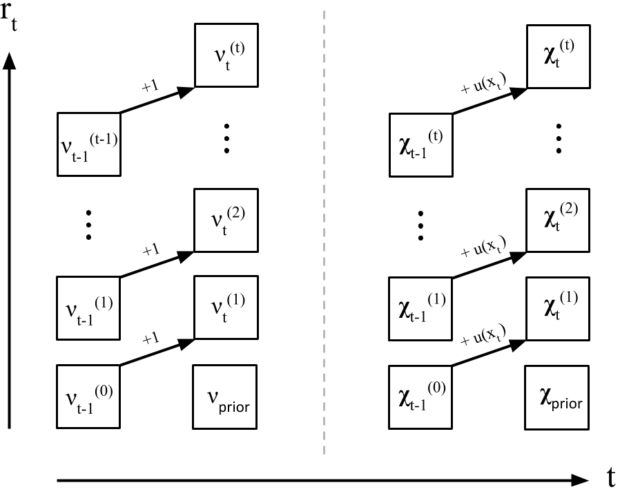
At each time point $t$, we want to model a new possible run-length. In this case, each parameter value is just its prior. Otherwise, we compute ${\nu }_t^{(\ell )}$ and ${\mathbf{\chi }}_t^{(\ell )}$ for each run length value $r_t=\ell$ by message-passing up the trellis. Formally,

$$\begin{array}{rl}{\nu }_t^{(0)}& ={\nu }_{\text{prior}}\\ {\mathbf{\chi }}_t^{(0)}& ={\mathbf{\chi }}_{\text{prior}}\\ {\nu }_t^{(\ell )}& ={\nu }_{t-1}^{(\ell -1)}+1\\ {\mathbf{\chi }}_t^{(\ell )}& ={\mathbf{\chi }}_{t-1}^{(\ell -1)}+u(x_t).\end{array}\text{\hspace{1em}(6)}$$

Changepoint prior

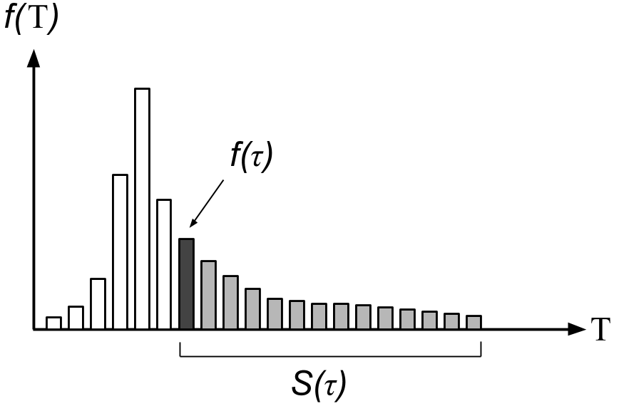
The changepoint prior allows us to encode our knowledge about our data’s changepoints into the model. Let $\mathrm{T}$ be a discrete, nonnegative random variable for the current run length. Let $f(\tau )$ denote the probability that the current run length is $\tau$. Let $S(\tau )$ be the survival function at $\tau$, which is the probability that $\mathrm{T}$ takes a value greater than $\tau$ or

$$S(\tau )=\mathbb{P}\{\mathrm{T}\ge \tau \}=\sum _{{\tau }^{\prime }=\tau }^{\infty }f({\tau }^{\prime })$$

Then hazard function $H(\tau )$ is

$$H(\tau )=\frac{f(\tau )}{S(\tau )}.$$

The hazard function quantifies the answer to the question: “Provided a changepoint has not occurred by run length $\tau$, what is the probability that it will occur at $\tau$?” The actual form of the hazard function clearly depends on the distribution of $\mathrm{T}$ (Figure $4$).

Figure 4. Diagram of the probability $H(\tau )$ for a hypothetical prior distribution $f(\tau )$.

Our modeling assumption is that our changepoint prior is

$$p(r_t\mid r_{t-1})=\{\begin{array}{ll}H(r_{t-1}+1)& \text{if rt=0}\\ 1-H(r_{t-1}+1)& \text{if rt=rt−1+1}\\ 0& \text{otherwise}.\end{array}\text{\hspace{1em}(7)}$$

For Equation $7$, we only need to compute two cases. The first case is the probability of a changepoint, which is just the hazard function. The second case is the probability that a changepoint does not occur, which is just one minus the probability of a changepoint. This prior is computationally efficient because we only have two cases with nonzero mass, and we only need to compute the hazard function once to compute both cases.

If $\mathrm{T}$ is a geometric random variable with a probability of success $p$, then $H(\tau )=p$ (Forbes et al., 2011). This kind of process is called memoryless because the hazard function does not depend on time.

Initial conditions

Earlier, we punted on discussing the initial conditions of our recursive algorithm,

$$p(r_0=0,{\mathbf{x}}_{1:t}=\varnothing )=p(r_0=0).$$

We now have the notation to address this question. We have two scenarios. The first scenario is that a changepoint occurred just before the first data point is observed or $p(r_0=0)=1$. This may not be the most realistic modeling assumption, but it is simple to implement.

The second scenario is that the first changepoint is in the future but we have access to some recent data. The example Adams gives is that of climate change. We have access to historic and current climate data and hypothesize that a changepoint will occur in the future. In this case, the prior over the initial run length is the normalized survival function

$$p(r_0=\tau )=\frac{1}{Z}\sum _{{\tau }^{\prime }=\tau +1}^{\infty }f({\tau }^{\prime })$$

where $Z$ is an appropriate normalizing constant. In words, this is all the mass in the future (note the sum starts at $\tau +1$, not $\tau$) divided by all the mass of the distribution $f(\cdot )$. The greater the value of $\tau$, the more mass the sum accumulates or the higher the probability that a changepoint will occur by some large $\tau$.

Sequential inference algorithm

We are now prepared to understand Bayesian online changepoint detection in algorithmic detail. This algorithm estimates the RL posterior distribution and performs prediction at each time point $t$. Let’s walk through the paper’s Algorithm $1$ with annotations as needed:

1. Set priors and initial conditions.

   $$\begin{array}{rl}p(r_0)& =\{\begin{array}{ll}1& \text{if changepoint at time t=0}\\ p(r_0=\tau )& \text{else}\end{array}\\ {\nu }_1^{(0)}& ={\nu }_{\text{prior}}\\ {\mathbf{\chi }}_1^{(0)}& ={\mathbf{\chi }}_{\text{prior}}\\ t& =1.\end{array}$$

2. Observe new datum $x_t$.

3. Compute UPM predictive probabilities. This calculation is for each possible run length value $\ell ,$

   $${\pi }_{t-1}^{(\ell )}=p(x_t\mid {\nu }_{t-1}^{(\ell )},{\mathbf{\chi }}_{t-1}^{(\ell )}).$$

   At time $t-1$, there are $t$ possible run lengths; we forward message-pass the mass for these values up the trellis to compute the UPM predictive over $x_t$; therefore there are $t$ probabilities ${\pi }_{t-1}^{(\ell )}$.

4. Compute growth probabilities. The growth probabilities are the probabilities $p(r_t=r_{t-1}+1,{\mathbf{x}}_{1:t})$ for each possible run length value. To compute the probability for a specific value $r_t=\ell$, Equation $3$ is

   $$p(r_t=\ell ,{\mathbf{x}}_{1:t})=p(r_{t-1},{\mathbf{x}}_{1:t-1}){\pi }_{t-1}^{(\ell )}(1-H(r_{t-1})).$$

   Note that there is no sum over $r_{t-1}$ because for a given run length, the only valid “growth value” is $r_{t-1}=\ell -1$.

5. Compute changepoint probability. The changepoint probability is the probability that the run length drops to $0$. Again using Equation $3$, we see

   $$p(r_t=0,{\mathbf{x}}_{1:t})=\sum _{r_{t-1}}p(r_{t-1},{\mathbf{x}}_{1:t-1}){\pi }_{t-1}^{(\ell )}H(r_{t-1}).$$

   In this case we have a sum over $r_{t-1}$ because $r_{t-1}$ can take any value between $0$ and $t$.

6. Compute the evidence. This is just the normalizer in Equation $2$.

7. Compute the RL posterior. Equation $2$.

8. Update sufficient statistics. Equation $6$.

9. Perform Prediction. Equation $1$.

10. Set $t=t+1$. Return to Step 2.

A complete example

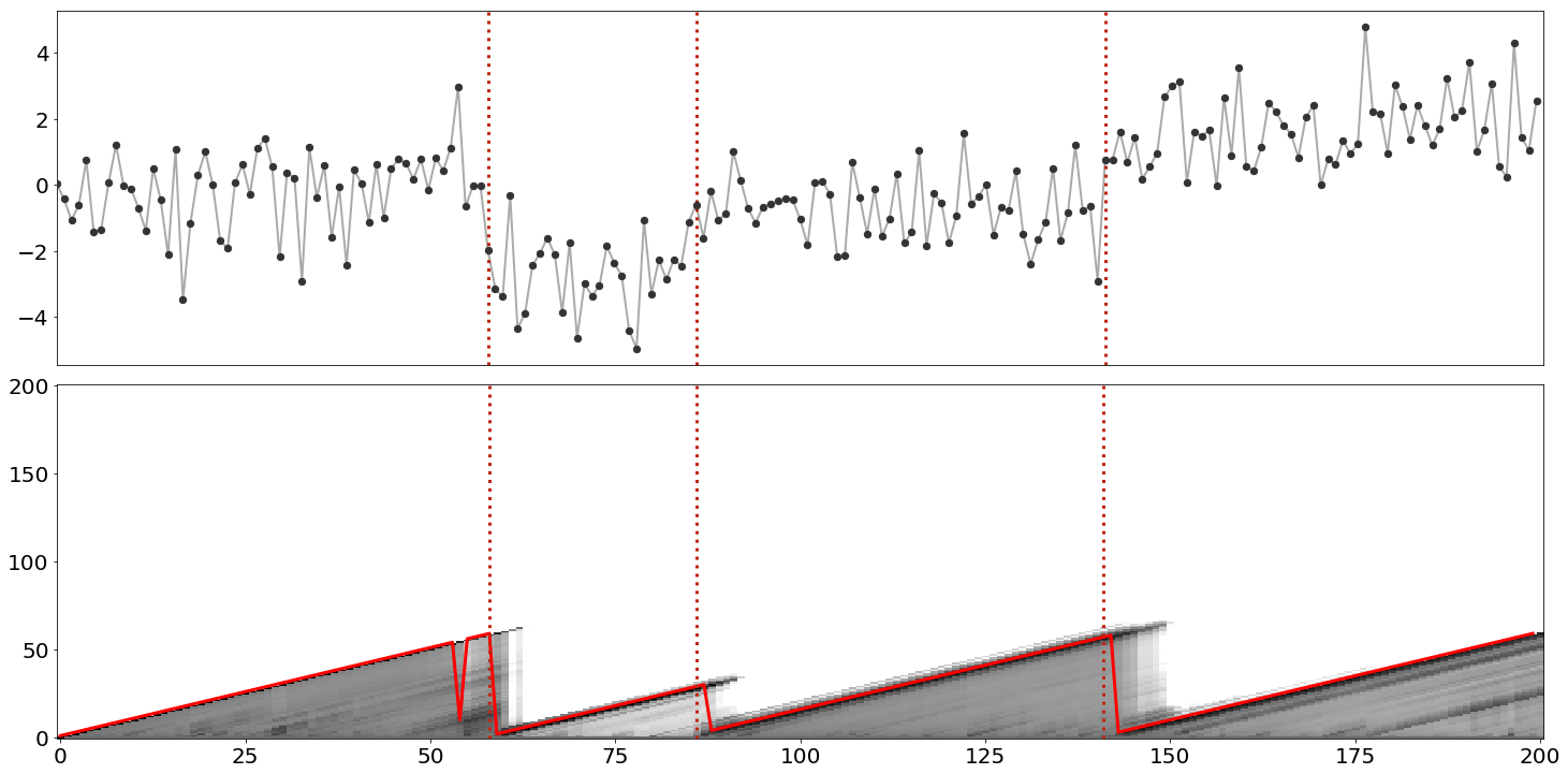
Now let’s work through a complete example and implementation of the algorithm. Consider the sequence of $T=200$ i.i.d. observations, $\mathcal{D}=\{{\mathbf{x}}_t{\}}_{t=1}^T$, in Figure $5\text{a}$. The groundtruth changepoints are denoted with red dashed lines. We might guess that these data look approximately Gaussian distributed and that while the mean $\mu$ sometimes changes, the variance ${\sigma }^2$ looks fairly consistent. Thus, to model these data, let’s use a Gaussian model with unknown $\mu$ and fixed precision $\lambda =1/{\sigma }^2$. The posterior predictive (the UPM predictive) for this model is

$$p(\hat{x}\mid \mathcal{D})=\mathcal{N}(\hat{x}\mid {\mu }_T,\frac{1}{\lambda }+\frac{1}{{\lambda }_T})$$

where $\hat{x}\in \mathbb{R}$ is a new observation and ${\mu }_T$ and ${\lambda }_T$ are defined as

$$\begin{array}{rl}{\mu }_T& =\frac{\frac{{\mu }_{\text{prior}}}{\lambda }+\frac{{\sum }_{t=1}^T{x}_t}{{\lambda }_{\text{prior}}}}{\frac{T}{{\lambda }_{\text{prior}}}+\frac{1}{\lambda }}\\ & \\ {\lambda }_T& ={\lambda }_{\text{prior}}+T\lambda \end{array}$$

See my post on Bayesian Inference for the Gaussian or (Murphy, 2007) for a complete derivation. To make the algebra easier, assume that $\lambda ={\lambda }_{\text{prior}}=1$; then we have

$$\begin{array}{rl}{\mu }_T& =\frac{{\mu }_{\text{prior}}+{\sum }_{t=1}^T{x}_t}{T+1}\\ & \\ {\lambda }_T& ={\lambda }_{\text{prior}}+T\end{array}$$

In changepoint detection, the number of samples $T$ is just the current time point $t$. So the parameter updates for ${\mu }_t^{(\ell )}$ and ${\lambda }_t^{(\ell )}$ as $t$ increases are

$$\begin{array}{rl}{\mu }_0^{(\ell )}& ={\mu }_{\text{prior}}^{(\ell )}\\ {\mu }_1^{(\ell )}& =\frac{{\mu }_0+x_1}{2}\\ {\mu }_2^{(\ell )}& =\frac{2{\mu }_1+x_2}{3}\\ {\mu }_3^{(\ell )}& =\frac{3{\mu }_2+x_3}{4}\\ & \dots \\ & \\ & \\ {\lambda }_0^{(\ell )}& ={\lambda }_{\text{prior}}^{(\ell )}\\ {\lambda }_1^{(\ell )}& =1+{\lambda }_1^{(\ell )}\\ {\lambda }_2^{(\ell )}& =1+{\lambda }_2^{(\ell )}\\ {\lambda }_3^{(\ell )}& =1+{\lambda }_3^{(\ell )}\\ & \dots \end{array}$$

In both instances, the parameter update is a simple function of the previous parameters and the next data point.

Figure 5. (Top) Synthetic data generated from a Gaussian distribution with fixed variance and a changing mean. Groundtruth changepoints are denoted with red dashed lines. (Bottom) The RL posterior at each time step using a logarithmic color scale. Darker indicates higher probability. The saw-toothed red line is the max probability at each time point.

To make things easy, let’s assume a memoryless hazard function, $H(\tau )=1/60$ because we see three changepoints in $200$ data points. The actual changepoint probability I used to generate the data was $1/80$. It is beyond the scope of this post, but clearly this hazard function is an important hyperparameter.

Now we are ready for code. While we have leveraged a lot of conceptual machinery, the code is strikingly simple:

import numpy as np
from   scipy.stats import norm


R        = np.zeros((T+1, T+1))
R[0, 0]  = 1
max_R    = np.empty(T+1)
max_R[0] = 1

H           = 1/60
mu_params   = np.array([mu0])
lamb_params = np.array([lamb0])

rl_pred = lambda x, mu, lamb: norm.pdf(x, mu, 1/lamb + 1)

for t in range(1, T+1):
    x = data[t-1]

    pis = np.array([rl_pred(x, mu_params[i], lamb_params[i]) for i in range(t)])

    R[t, 1:t+1] = R[t-1, :t] * pis * (1-H)
    R[t, 0]     = sum(R[t-1, :t] * pis * H)
    R[t, :]    /= sum(R[t, :])

    max_R[t] = np.argmax(R[t, :])

    offsets     = np.arange(1, t+1)
    mu_params   = np.append([mu0], (mu_params * offsets + x) / (offsets + 1))
    lamb_params = np.append([lamb0], lamb_params + 1)

Note that the above code is a didactic snippet, i.e. you cannot paste this into a file and run it. For a complete example, see my GitHub. We can visualize the results of this algorithm by plotting both the RL posterior and the max posterior value (Figure $5\text{b}$).

Finally, note that Bayesian online changepoint detection is a modular algorithm because both computing the UPM predictive and updating the parameters could be methods on a distribution class that keeps track of the state of its own parameters. Adams notes this in the paper by saying that the framework delineates “between the implementation of the changepoint algorithm and the implementation of the model.”

Conclusions

Bayesian online changepoint detection is a modular Bayesian framework for online estimation of changepoints. It models changes in the generative parameters of data by estimating the posterior over the run length, and it leverages conjugate-exponential models to achieve modularity and efficient parameter estimation. The method is Bayesian in that the changepoint prior allows us to encode knowledge about the world and it models uncertainty about $\mathbf{\theta }$, and it is online because it computes the RL posterior at each time step using only previously seen data.

This paper is from 2007, and I am not up-to-date on the literature on extending this work. However, I would guess that key areas for future work would be addressing the memory usage, which grows quadratically with $T$; robustly handling a misspecified model or prior; and developing approximate inference routines for non-conjugate models.

Acknowledgements

I thank Diana Cai for giving me an introductory overview of this model and providing working code and Ryan Adams for answering questions about the paper.